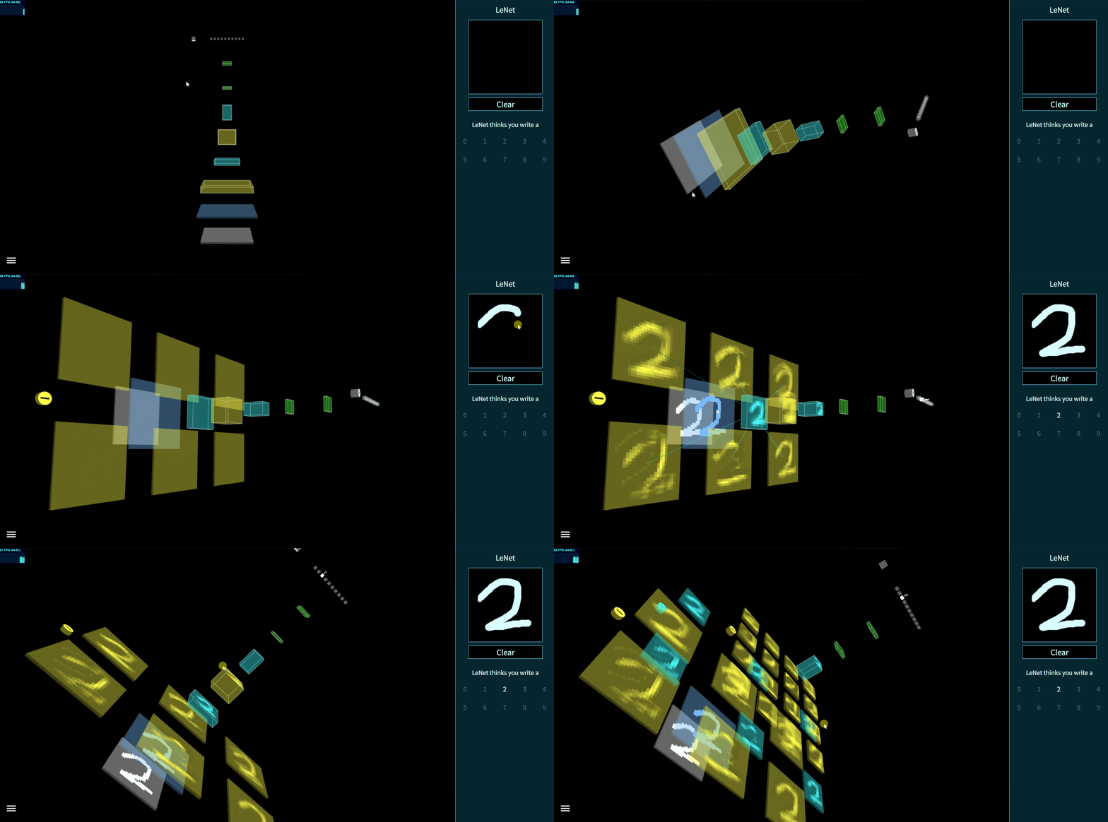
Nowadays, Deep Learning becomes more and more popular in many domains like Finance, E-Commerce. At OtoNhanh.vn, we employ Deep Learning to tackle the problems of Natural Language Processing to deal with the requests of the user in our site or of Computer Vision in the illustration of cars. In this blog, we will focus on the network architectures that we consider to use in our Computer Vision application. There will be 3 parts in this blog:
- Part 1: ConvNet and its principal elements
- Part 2: ConvNet architectures
- Part 3: Challenges and future vision
All the source codes in this blog base on TensorFlow in Python2.7
I. Convolutional Neural Network (ConvNet)
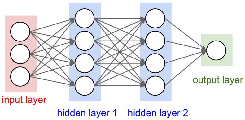
The heart of Deep Learning in Computer Vision is ConvNet, a sub-division of Neural Network designed specifically to cope with the images. Regular Neural Network is made of fully-connected layers: each unit from one layer have the access to every units from the previous layer, which leads to the explosion in the number of parameters of the network. For example, if we have a RGB image whose size is 200x200 as an input, each neuron in the first hidden layer will have 200x200x3 = 120000 weights to compute the output. This redundancy of the parameters is really a catastrophe for the training procedure: it doesn’t help to generalize the problems well and results in the slow convergence due to the large amount of the parameters.
In this context, Yann LeCunn developed a biologically-inspired neural network called ConvNet. ConvNet comprises 3 main types of layer: Convolutional Layer, Pooling Layer and Fully Connected Layer.
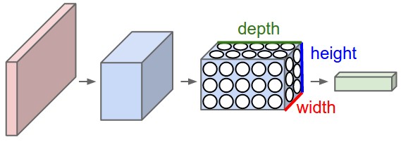
A ConvNet is made up of Layers. Every layer has a simple API: It transforms an input 3D volume to an output 3D Volume with some differentiable function that may or may not have parameters.
Convolutional Layer
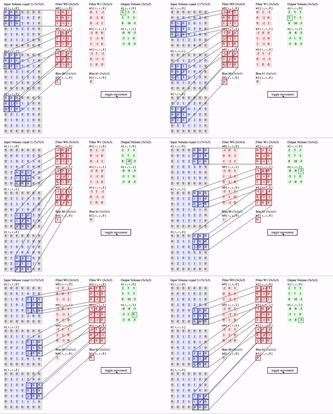
It plays the roles of feature detector in ConvNet. In more detailed, it computes the dot product of 3-D kernel with local region from input image. This sliding-window method can be considered as convolution operation, this is the origin of its name. Each kernel will detect a same feature in every region of the image and will send it to the higher layer to construct more delicate feature detector. After the convolution, we prefer to apply some sorts of activation function like ReLU or tanh… to adapt to the non-linearity.
Convolution has been used previously with some man-made filter like Laplace or Sobel to detect feature in the image, however, ConvNet proposes a way to learn the filters automatically.
Pooling Layer
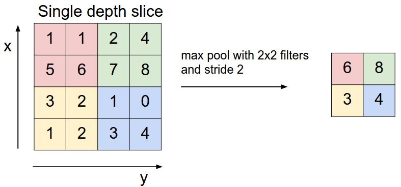
The most two popular pooling operation are average pooling and max pooling. This layer is used to achieve the invariance during the training. It means that if we modify the input a little bit, it won’t affect the overall result much. This invariance is very important in the task of classification as we may capture the same object but from the different pose or it may have capture the noise as well.
However, the way it achieve the invariance by losing the information raises a lot of arguments in the Deep Learning community. Recently, G.Hinton, a “god father” in this domain, has publicized his research about Capsule Net, a method to achieve the pose invariance without using pooling.
Fully-Connected Layer
At the end of ConvNet, we always put this layer, accompanied by a softmax loss function in case of multi-classification. It will measure the score for each label so that we could choose the label for the input image.
Generally speaking, Convolutional Layer, Pooling Layer and Fully-Connected Layer are the principal components of ConvNet in the image classification task. To make use these layers at its best, the researchers in Deep Learning community try to construct different network architectures. The arrival of ConvNet has changed the fundamental tasks of Computer Vision from feature engineering to network engineering to find the best representation for the classification. One of the most popular benchmark is the ImageNet challenge. To further boost the performance of ConvNet, the researchers also introduces some secondary components like Batch Normalization, Local Response Normalization, Dropout… In the next part, we will concentrate on the architectures that we have implemented in our business.
A very cool illustration
