In this part, I will discuss many famous architectures of ConvNet which are employed in image classification throughout the years.
1. AlexNet
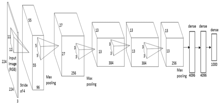
It is developed by Alex Krizhevsky and al.. It was submitted to the ImageNet Challenge in 2012 and really made an echo in Deep Learning society by its superiority in the contest. In fact, it is pretty similar to the famous LeNet but bigger and deeper.
Furthermore, it introduced local response normalization to improve the performance and some techniques like data augmentation or dropout to enhance the generalization. Also, it provides us an implementation technique to carry out the training in limited hardware.
Detail of AlexNet architecture used in ImageNet Challenge:
-
There are 8 main layers in AlexNet: the first five layer are Convolutional Layer and their dependencies. The remaining three layers are the fully-connected layer. The outputs of the last fully-connected layer are brought to 1000-way soft-max classifier.
-
The kernel of the second, fourth and fifth convolutional layer are connected to the kernel from the previous layer. Local response normalization follows only the first two convolutional layer. Max pooling operation follows both normalization layer and the fifth convolution layer. ReLU non-linearity is applied to every output of convolutional layer and fully connected layer.
- One thing to notice: The above architecture is suitable for ImageNet whose size is large, for other datasets like MNIST or CIFAR10, we have to reduce some layers to avoid Vanish Gradient.
Source code for AlexNet:
with tf.device('/gpu:0'):
    with tf.variable_scope('1st_conv'):
        net = slim.conv2d(images, num_outputs=96, kernel_size=[7, 7], stride=1)
        net = conv_2d(images, 96, [7, 7], [1, 1])
        net = tf.nn.lrn(net, alpha=1.e-3, beta=0.75, bias=2)
        net = max_pooling(net, [2, 2], [1, 1])
    with tf.variable_scope('2nd_conv'):
        net = slim.conv2d(net, num_outputs=256, kernel_size=[5, 5], stride=2)
        net = conv_2d(net, 256, [3, 3], [2, 2])
        net = tf.nn.lrn(net, alpha=1.e-3, beta=0.75, bias=2)
        net = max_pooling(net, [2, 2], [1, 1])
    with tf.variable_scope('3rd_conv'):
        net = slim.conv2d(net, num_outputs=384, kernel_size=[3, 3], stride=2)
        net = conv_2d(net, 384, [3, 3], [2, 2])
        net = tf.nn.lrn(net, alpha=1.e-3, beta=0.75, bias=2)
        net = max_pooling(net, [2, 2], [1, 1])
        net = fully_connected(net, 2048, activation=None)
        net = slim.fully_connected(net, num_outputs=4096, activation_fn=None)
    with tf.variable_scope('1st_bn'):
        net = batch_norm(net, mode='train')
        net = slim.batch_norm(net)
        net = tf.nn.tanh(net)
        net = slim.fully_connected(net, num_outputs=2048, activation_fn=None)
        net = fully_connected(net, 2048, activation=None)
    with tf.variable_scope('2nd_bn'):
        # net = batch_norm(net, mode='train')
        net = slim.batch_norm(net)
    net = tf.nn.tanh(net)
    net = fully_connected(net, 10, activation='None')
    net = slim.fully_connected(net, num_outputs=10, activation_fn=None)
    loss_op = tf.nn.sparse_softmax_cross_entropy_with_logits(
        labels=labels,
        logits=net
    )
Its detailed architecture can be found in the paper ImageNet Classification with Deep Convolutional Neural Networks.
2. VGG-Net
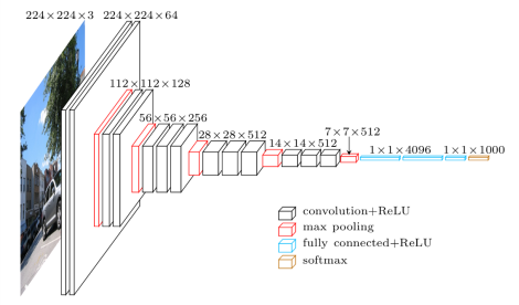
This architecture is, from my point of view, a deeper version of AlexNet. Its main contribution is that a better performance of the network can be achieved by simply increasing its layers for more sophisticated representation. Furthermore, VGG-style strategy of repeating layers of the same shape helps for isolating a few factors and extending to any large number of transformation. This strategy is inherited profoundly by ResNext.
with slim.arg_scope(arg_scope):
    x = slim.conv2d(x, 64, 3, 1, activation_fn=tf.nn.relu, scope='conv1_1')
    x = slim.conv2d(x, 64, 3, 1, activation_fn=tf.nn.relu, scope='conv1_2')
    x = slim.maxpool2d(x, 2, 2, padding='SAME', scope='pool1')

    x = slim.conv2d(x, 128, 3, 1, activation_fn=tf.nn.relu, scope='conv2_1')
    x = slim.conv2d(x, 128, 3, 1, activation_fn=tf.nn.relu, scope='conv2_2')
    x = slim.max_pool2d(x, 2, 2, padding='SAME', scope='pool2')

    x = slim.conv2d(x, 256, 3, 1, activation_fn=tf.nn.relu, scope='conv3_1')
    x = slim.conv2d(x, 256, 3, 1, activation_fn=tf.nn.relu, scope='conv3_2')
    x = slim.conv2d(x, 256, 3, 1, activation_fn=tf.nn.relu, scope='conv3_3')
    x = slim.max_pool2d(x, 2, 2, padding='SAME', scope='pool3')

    x = slim.conv2d(x, 512, 3, 1, activation_fn=tf.nn.relu, scope='conv4_1')
    x = slim.conv2d(x, 512, 3, 1, activation_fn=tf.nn.relu, scope='conv4_2')
    x = slim.conv2d(x, 512, 3, 1, activation_fn=tf.nn.relu, scope='conv4_3')
    x = slim.max_pool2d(x, 2, 2, padding='SAME', scope='pool4')

    x = slim.conv2d(x, 512, 3, 1, activation_fn=tf.nn.relu, scope='conv5_1')
    x = slim.conv2d(x, 512, 3, 1, activation_fn=tf.nn.relu, scope='conv5_2')
    x = slim.conv2d(x, 512, 3, 1, activation_fn=tf.nn.relu, scope='conv5_3')
    x = slim.max_pool2d(x, 2, 2, padding='SAME', scope='pool5')

    pool_shape = x.get_shape().as_list()
    flat_size = pool_shape[1] * pool_shape[2] * pool_shape[3]
    x = tf.reshape(x, [pool_shape[0], flat_size])

    x = slim.fully_connected(x, 4096, activation_fn=tf.nn.relu, scope='fc1')
    x = slim.fully_connected(x, 4096, activation=tf.nn.relu, scope='fc2')

    if self.model_cfg['is_training']:
        if dropout_prob > 0.:
            x = tf.nn.dropout(x, 1.0 - self.model_cfg['dropout_prob'])

    logits, probs = predict_layer(x, num_classes, using_logistic_regression)
Its detailed architecture can be found in the paper Very deep convolutional networks for large-scale image recognition.
3. Inception
Along with VGGNet, Inception is also a contestant in the 2014 ILSVRC who gained much attention from the community. While VGGNet gives us a simple way to reinforce the result by stacking more layers, Inception gives us many new notions which, in my opinion, inspires many successors. Inception architecture sticks to a very famous meme in the internet:

There are two papers about this architecture that worth noticing:
Going Deeper with Convolutions
Rethinking the Inception Architecture for Computer Vision
Personally, I recommend you to take time with the second paper, it gives us some insights about Inception. Now I will summarize the ideas of the paper:
General Design Principles
-
Avoid representational bottlenecks: We shouldn’t reduce the size as well as the dimension of the input too abruptly, especially in the first layers. The representation size ought to be shrank mildly throughout the network in order to avoid the loss of information.
-
Higher dimensional representations are easier to process: Adding more filters per tile is encouraged for the purpose of faster training.
-
Spatial aggregation can be done over lower dimensional embeddings without much or any loss in representational power: Considering adjacent layers are highly correlated, it results in much less loss of information during dimension reduction. So why not reducing the dimension for a faster learning?
-
Balance the width and depth of the network: We should increase both the depth of the network and the number of filters per stage for the optimal improvement.
Factorizing Convolution
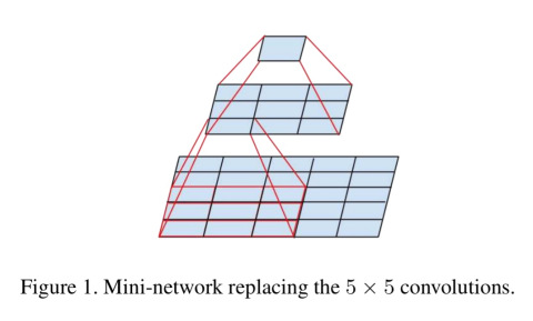
In my own experience, before reading this paper, I had always had an impression that a larger filter size will lead to a faster training due to the fact that larger filter size make smaller feature maps. However, it turns out that instead of using a large filter, we should factorize it into smaller filter layers. For instance, two 3x3 layers are more preferable than a 5x5 filter.
Furthermore, although it seem logical when we don’t introduce ReLU layer between the two small convolutional layer to simulate the large layer at its best, the author advised us to employ the ReLU layer after each convolution.
Auxiliary Classifiers
Inception also introduces a new concept of auxiliary classifiers. We add some classifiers at the intermediate layers: Their loss is added to the total loss with a specific weights. In the inference, these classifiers are discarded. They act as the regularizer and also a way to combat vanishing gradient. However, it is proved that their contribution is quite limited, and in most case, just a secondary classifier is sufficient.
Grid Size Reduction
Traditionally, to reduce the size of the feature map, we use pooling operator before entering a module, which is contrast to the principle of avoiding representational bottlenecks. We may reverse the order by executing the module first and then applying the pooling, however, it is computationally expensive.
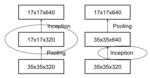
The author proposed to use concatenation as a way to bypass the bottleneck but still reduce the size:
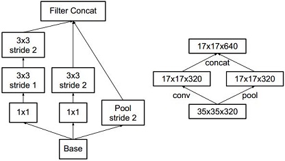
Inception Architecture
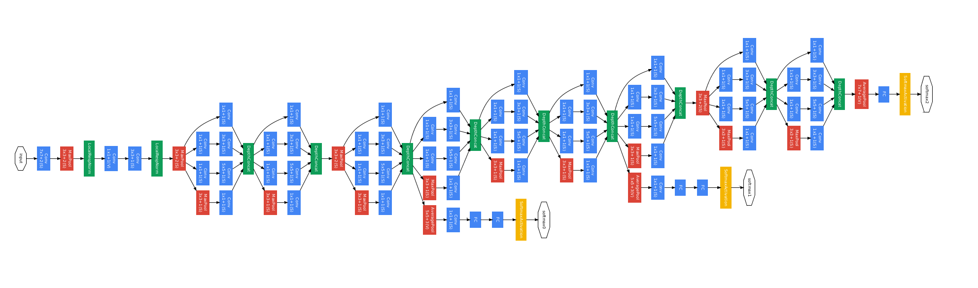
Its core element is Inception module. In this module, we use different filter size to the same input and combine the feature map using concatenation. In the module, we also implement some above tricks to improve the training process.
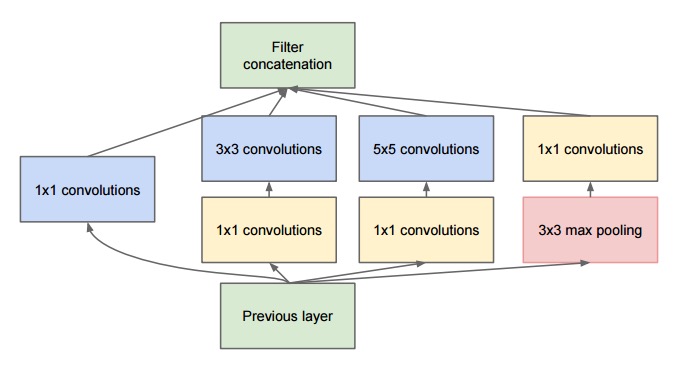
with tf.variable_scope('Mixed_7a'):
    with tf.variable_scope('Branch_0'):
        tower_conv = slim.conv2d(x, 256, 1, scope='Conv2d_0a_1x1')
        tower_conv_1 = slim.conv2d(tower_conv, 384, 3, stride=2,
                                    padding='VALID', scope='Conv2d_1a_3x3')
    with tf.variable_scope('Branch_1'):
        tower_conv1 = slim.conv2d(x, 256, 1, scope='Conv2d_0a_1x1')
        tower_conv1_1 = slim.conv2d(tower_conv1, 288, 3, stride=2,
                                    padding='VALID', scope='Conv2d_1a_3x3')
    with tf.variable_scope('Branch_2'):
        tower_conv2 = slim.conv2d(x, 256, 1, scope='Conv2d_0a_1x1')
        tower_conv2_1 = slim.conv2d(tower_conv2, 288, 3,
                                    scope='Conv2d_0b_3x3')
        tower_conv2_2 = slim.conv2d(tower_conv2_1, 320, 3, stride=2,
                                    padding='VALID', scope='Conv2d_1a_3x3')
    with tf.variable_scope('Branch_3'):
        tower_pool = slim.max_pool2d(x, 3, stride=2, padding='VALID',
                                        scope='MaxPool_1a_3x3')
    x = tf.concat(3, [tower_conv_1, tower_conv1_1,
                        tower_conv2_2, tower_pool])
Basically, it is the concept of Inception architecture that we want to introduce. In the paper, they also talk about a regularization technique called Label Smoothing, but it is out of scope of this article.
4. ResNet
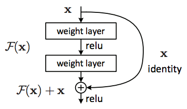
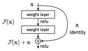
Unlike some above architectures when they simply increase the depth of the network to enhance the performance, this time, Kaiming He and al have done something ground-breaking to improve the classification. It really makes a way for us to train hyper deep network with compelling performance. After VGGNet, Deep Learning community has the impression that a deeper network will definitely bring us to a better performance. Nevertheless, Kaiming He discovered that it is only true to some extent, after that the error rate may be up. This fact is against our intuition: A deeper architecture must have a more representational power or at least have a same performance with the shallow one in case the added layers are identity mappings. Based on that observation, he wondered that instead of mapping the function \(f(x)\), it may be easier to map the residual function \(h(x) = f(x) - I\) (in which I is the identity mapping). After obtaining the approximation \(\hat{h}\), we could easily add I back to get the representation \(\hat{f}\) of the underlying function \(f(x)\).
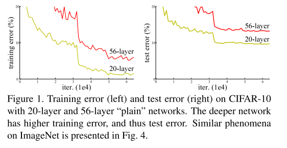
To be more precise, in the original paper, the authors indicated that it exists the degradation in performance when we deepen the network. Overfitting is not the cause since the training error is also higher in case of deeper network.
Kaiming He had an impression that the neural networks have difficulties in mapping the identity function. With residual blocks, when identity mapping is sufficient, the neural networks may drive the weights of theirs layers towards zero so as to approach the identity mappings.
In practice, it is rare that identity mappings are optimal but according to the authors:
… our reformulation may help to precondition the problem. If the optimal function is closer to an identity mapping than to a zero mapping, it should be easier for the solver to find the perturbations with reference to an identity mapping, than to learn the function as a new one
Based on our experience, ResNet is still one of the most powerful Deep Learning architecture in term of error rate and efficiency computation.
Source code for Residual Block:
def bottleneck_residual(x,
                    nin_feature_maps,
                    nout_feature_maps,
                    strides,
                    activate_before_residual=False,
                    is_training=True,
                    relu_leakiness=0.0,
                    name='bottleneck_v2'):
    """Bottleneck residual unit with 3 sub layers"""
    with tf.variable_scope(name):
        if activate_before_residual:
            x = slim.batch_norm(x, is_training=is_training, scope='preact')
            x = chappiedl.nn.leaky_relu(x, relu_leakiness)
            orig_x = x
        else:
            orig_x = x
            x = slim.batch_norm(x, is_training=is_training, scope='preact')
            x = chappiedl.nn.leaky_relu(x, relu_leakiness)

        x = slim.conv2d(x,
                        nout_feature_maps / 4,
                        (1, 1),
                        strides,
                        biases_initializer=None,
                        activation_fn=None,
                        scope='conv1')
        x = slim.batch_norm(x, is_training=is_training, scope='conv1/BatchNorm')
        x = chappiedl.nn.leaky_relu(x, relu_leakiness)

        x = slim.conv2d(x,
                        nout_feature_maps / 4,
                        (3, 3),
                        (1, 1),
                        biases_initializer=None,
                        activation_fn=None,
                        scope='conv2')
        x = slim.batch_norm(x, is_training=is_training, scope='conv2/BatchNorm')
        x = chappiedl.nn.leaky_relu(x, relu_leakiness)

        x = slim.conv2d(x,
                        nout_feature_maps,
                        (1, 1),
                        stride=(1, 1),
                        activation_fn=None,
                        scope='conv3')

        if nin_feature_maps != nout_feature_maps:
            orig_x = slim.conv2d(orig_x,
                                nout_feature_maps,
                                (1, 1),
                                stride=strides,
                                scope='shortcut')

        x += orig_x

    return x
Its detailed architecture can be found in the paper Deep Residual Learning for Image Recognition.
5. ResNeXt
As ResNet performance in 2015 ILSVRC blew people’s mind, its architecture is getting studied heavily and some refinements have been made in the architecture. ResNeXt is one of them. Its core element is called ResNext building block:
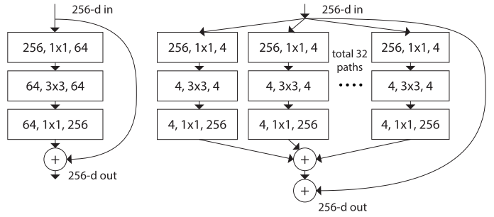
As you can see, ResNext building block is a fusion of residual block and Inception block. ResNeXt resembles Inception that input will go though several convolution paths, the outputs of these paths are merged by the addition, unlike the concatenation in Inception. Before leaving the block, it will be added with the input like the ResNet in order to produce the overall output of the block. All the paths in the ResNeXt block share the same topology, which helps to simplify the hyper-parameters tuning.
The transformations to be aggregated are all of the same topology. This design allows us to extend to any large number of transformations without specialized design.
The authors argue that this architecture is more easily tuned than its predecessors since it has a simple paradigm and only one hyper-parameter to be adjusted. They also state that modifying the cardinality is more effective than modifying width/depth of the network.
def _resneXt_bottleneck_B(
            x,
            nin_feature_maps,
            nout_feature_maps,
            strides,
            base_width=None,
            cardinality=None,
            is_training=True,
            relu_leakiness=0.0):
    origin_x = x
    d = (nout_feature_maps * base_width / 128)
    c = cardinality
    with tf.variable_scope('bottleneck_residual'):
        x = slim.conv2d(x,
                        d,
                        (1, 1),
                        strides=(1, 1),
                        activation_fn=None,
                        biases_initializer=None,
                        scope='conv1')

        x = slim.batch_norm(x, is_training=is_training, scope='conv1/BatchNorm')
        x = chappiedl.nn.leaky_relu(x, relu_leakiness)

        with tf.variable_scope('conv2'):
            x = _split(x, c,
                       strides=strides,
                       is_training=is_training,
                       relu_leakiness=relu_leakiness)

        x = slim.conv2d(x,
                        nout_feature_maps,
                        (1, 1),
                        strides=(1, 1),
                        activation_fn=None,
                        scope='conv3')
        x = slim.batch_norm(x, is_training=is_training, scope='conv3/BatchNorm')

        origin_x = _shortcut(origin_x,
                             nin_feature_maps,
                             nout_feature_maps,
                             strides,
                             is_training=is_training,
                             shortcut_type='B')
        x += origin_x
        x = chappiedl.nn.leaky_relu(x, relu_leakiness)

    return x
More details about the implementation can be found in the paper Aggregated Residual Transformations for Deep Neural Networks
6. DenseNet
DenseNet is the latest Deep Learning architecture published by Gao Huang and al.. From their point of view, the degradation in error rate when the network becomes deeper comes from the fact that the information from input vanishes while passing the layers. So we consider that the shortcut in the residual blocks from ResNet is one way to maintain the information from the input till the end of the network.
The authors of DenseNet pushed the idea of ResNet to its limit. To maximize the information flow between layers in the network, they divide DenseNet into the dense blocks in which all the layers are directed connected. However, in contrast to ResNet, DenseNet combines the feature map not by adding them but by concatenating them. Due to its dense connection in the block, they named this architecture as Dense Convolution Network (DenseNet)
As I have stated above, Dense Block is the core element of Dense Convolution Network.

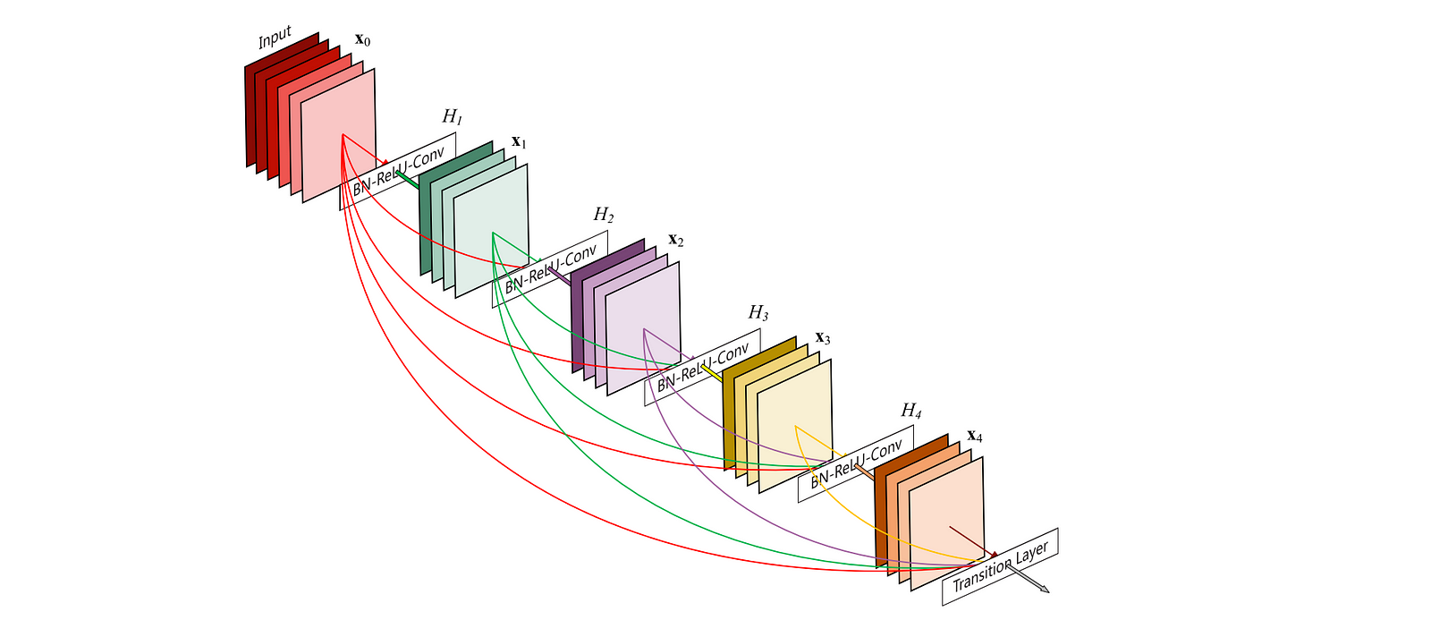
As you can see, Dense Block is divided again into several groups of (1x1 convolution and 3x3 convolution). The number of groups is block depth. The input of each group is the concatenation of its previous group’s output. 1x1 convolution is optional; if we equip this dimension reduction to a group, we could call it bottleneck layer. The below code is the Dense Block we implement in our classification.
def dense_block(
    incoming, block_depth,
    growth_rate, scope,
    drop_out,
    keep_prob=None,
    is_training=True):
    """ Dense block

    :param incoming: block input
    :param block_layers: number of block layers
    :param growth_rate: Growth rate
    :param scope: Scope of dense block
    :param keep_prob: (1 - keep_prob) dropout prob
    :param is_training: Is training process or not
    :return:
    """
    x = incoming
    with tf.variable_scope(scope):
        for i in range(block_depth):
            conn = x
            with tf.variable_scope('%d_th_layer' % (i+1)):
                with tf.variable_scope('sub1'):
                    x = slim.batch_norm(x, is_training=is_training, fused=True)
                    x = tf.nn.relu(x)
                    x = slim.conv2d(x, 4 * growth_rate, 1, 1, activation_fn=None, padding='VALID')
                    if drop_out:
                        x = tf.nn.dropout(x, keep_prob)
                with tf.variable_scope('sub2'):
                    x = slim.batch_norm(x, is_training=is_training, fused=True)
                    x = tf.nn.relu(x)
                    x = slim.conv2d(x, growth_rate, 3, 1, activation_fn=None)
                    if drop_out:
                        x = tf.nn.dropout(x, keep_prob)
            x = tf.concat([x, conn], 3)
    return x
Between the Dense Blocks, we add Transition Layer to further improve the model compactness. If the previous Dense Block produces \(m\) feature maps, we let the Transition Layer generate \(\theta m\), \(\theta \in\) [0, 1].
def transition_block(
    incoming, compression_rate, drop_out,
    keep_prob, scope, is_training=True):
    """Transition block
    :param incoming: block input
    :param compression_rate: Compression rate
    :param keep_prob: (1 - keep_prob)
    :param is_training: Is training process
    """
    imcoming_channel = incoming.get_shape().as_list()[3]
    with tf.variable_scope(scope):
        x = slim.conv2d(incoming, int(compression_rate * imcoming_channel), 1, 1, activation_fn=None)
        if drop_out:
            x = tf.nn.dropout(x, keep_prob)
        x = slim.avg_pool2d(x, 2, 2)
    return x
Even though DenseNet seems potential, the implementation into production is quite complicated in aspect of training time and memory consumption. According to the author:
One of the reasons why DenseNet is less memory/speed-efficient than Wide ResNet, is that in our paper, we mainly aimed to compare the connection pattern between DenseNets (dense connection) and ResNets (residual connection), so we build our DenseNet models in the same “deep and thin” fashion as the original ResNets (rather than Wide ResNets). Based on our experiments, on GPUs, those “deep and thin” models are usually more parameter-efficient, but less memory/speed-efficient, compared with “shallow and wide” ones.
Backprop requires storing all layer’s outputs, therefore the number of such layers (and their respective output sizes) is the main culprit for memory bottlenecks.
So it seems that there is a trade-off between parameter efficiency and memory/speed efficiency. We choose
shallow and wide version in deployment.
Its detailed architecture can be found in the paper Densely Connected Convolutional Networks.