In the last blog about Distributed TensorFlow, we have provided some fundamental knowledge of Distributed Training in this framework. However, it is not enough if we want to apply it efficiently. Today, we will provide some additional tricks to make use of Distributed Computing better in OtoNhanh.vn.
I. Facebook’s tricks to train ImageNet faster
On June 8, 2017, the age of distributed deep learning began. On that day, Facebook released a paper showing the methods they used to reduce the training time for a convolutional neural network (RESNET-50 on ImageNet) from two weeks to one hour, using 256 GPUs spread over 32 servers.
Surely, the above statement is a bit exaggerated but it still indicates that this paper has helped to boost the performance of Distributed Deep Learning. In this part, let me introduce some insights of this paper. Back to Stochastic Gradient Descent, the heart of Deep Learning, the idea is to estimate the gradient of the loss function \(\bigtriangledown L\) using training input. There are two common strategies: Using all the training data to compute the gradient Batch Gradient Descent and randomly choosing a small subset of training data to compute the gradient Mini-batch Gradient Descent. The first method estimates the gradient more exactly but more computationally expensive. This trade-off is really popular in Deep Learning. Recently, people argue that mini-batch brings another advantage: it acts as a regularizer in training process: more accurate gradient means better adaptation to training set and to some extent, means a worse generalization.
While distributed synchronous SGD is now commonplace, no existing results show that validation accuracy can be maintained with mini-batches as large as 8192 or that such high-accuracy models can be trained in such short time.
Nonetheless, limiting the batch size is really a waste since the hardwares are more and more powerful and distributed computing is available. In this circumstance, Facebook tries to demonstrate the feasibility of and to communicate a practical guide to large-scale training with distributed synchronous stochastic gradient descent. In short, they aim to keep the validation error low in the shortest time while using a large batch-size to utilize Distributed Computing. The key idea is to modify the learning rate so that the training curves in the case of large batch-size imitate these of small batch-size.
Linear Scaling Rule
When the mini-batch size is multiplied by k, multiply the learning rate by k.
To interpret this rule, we come back to the fundamental expression of Gradient Descent:
Consider a network at iteration \(t\) with weight \(w_t\), and a sequence of \(k\) mini-batches \(\beta_j\) for \(0 \le j < k\) each of size \(n\). We want to compare the effect of executing \(k\) SGD iterations with small mini-batches \(\beta_j\) and learning rate \(\eta\) versus a single iteration with large mini-batch \(\cup_j\beta_j\) of size \(kn\) and learning rate \(\hat\eta\). In the first case, after \(k\) iterations of SGD, we have:
On the other hand, taking a single step with a large mini-batch and learning rate \(\hat\eta\) will result in:
\(\hat w_{t+1} = w_t - \hat\eta\frac{1}{kn} \sum_{j<k} \sum_{x\in\beta_j} \bigtriangledown l(x, w_t)\)
As we can see, there is unlikely that \(w_{t+k} = \hat w_{t+1}\). However, if we could guarantee that \(\bigtriangledown l(x, w_t+j) \approx \bigtriangledown l(x, w_t)\), we can set \(\hat\eta = k\eta\) to yield \(w_{t+k} \approx \hat w_{t+1}\). The assumption that \(\bigtriangledown l(x, w_t+j) \approx \bigtriangledown l(x, w_t)\) is strong and often does not hold, however, according to Facebook, this works really well in practice: not only the final accuracies stay similar, the learning curve match closely. There are two cases that we may not apply this rule: the initial training epochs when the network changes rapidly (we could use warmup strategy to address this issue) and \(k\) becomes enormous. The mini-batch size limit, according to Facebook, is \(~8k\) in ImageNet experiment.
Warmup
As we have discussed, the linear scaling rule breaks down in the early stage of learning when the network changes rapidly. Facebook thinks that this matter can be alleviated by using less aggressive learning rate at the start of the training. There are 2 types of warmup:
- Constant warmup:
We use a low constant learning rate during a first few training epochs. However, Facebook observed that strategy is not sufficient in case of large \(k\). Furthermore, an abrupt transition out of low learning rate can cause the training error to spike. So they propose the following gradual warmup.
- Gradual warmup:
In this setting, we gradually ramp up the learning rate from a small to large value. In practice, we start the learning rate from a value \(\eta\) and increase it by a constant amount at each iteration so that the learning rate could reach \(\hat\eta = k\eta\) after a number of epochs(normally 5 epochs). This setting avoids a sudden increase in the value of learning rate, allows a healthy convergence at the beginning of learning. After the warmup phase, we could go back to the original learning rate schedule.
II. Uber framework for Distributed Training
To begin with, Uber is one of the most active companies in the field of Deep Learning. They apply Deep Learning to pair the drivers and the customers. With the augmentation of the dataset, they invest strongly to increase the computational power of their Deep Learning engine. And Horovod is one of the most remarkable solutions of theirs. Horovod, in short, is a framework which helps to exploit the computational power of distributing system much more efficiently than standard Distributed TensorFlow.
Back to Distributed TensorFlow, we have to admit that there are many new concepts like: worker, parameter server, tf.ClusterSpec() etc.: it is hard for a newbie to understand fully and also hard for an expert to debug his program. So we are in need of a simpler wrapper.
Another issue is, the standard Distributed TensorFlow cannot exploit fully the hardware power.
Obviously, we cannot expect that the real performance can reach the theoretical one. However, according to the above illustration, we can’t ignore the fact that the conventional mechanism is wasting the hardware capacity. Motivated by Facebook’s paper, Uber open-sourced their distributed framework named Horovod in TensorFlow.
Message Passing Interface (MPI)
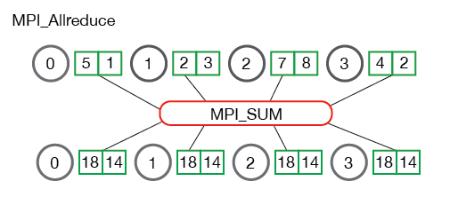
To understand the mechanism of Horovod, we have to study some MPI’s concept. Horovod core principles are based on MPI to aggregate the gradient. According to Facebook, in the deep learning network, each GPU has their own gradient and to update the parameters, we must combine these gradients. As the models grow complex and the computation capacity increases, it is hard to ignore the aggregation cost in the backprop. Message Passing Interface provides us a way to address the issue. Consider that we train a model on 4 servers with 4 GPUs in each.
- Size is the number of processes, in this case, 16. If GPUs are equipped with Hyper-Threading technology, there would be 32, but it is for the future.
- Rank is the unique process ID from 0 to 15.
- Local rank is the unique process ID within the servers. To sum up, each GPU has two kinds of ID.
- All-reduce is an operation which combines the gradients from the GPUs and distributes back to them.
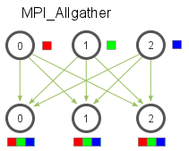
- All-gather is an operation that one process gathers data from the other processes.
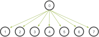
- Broadcast is an operation that diffuses the data from one process.
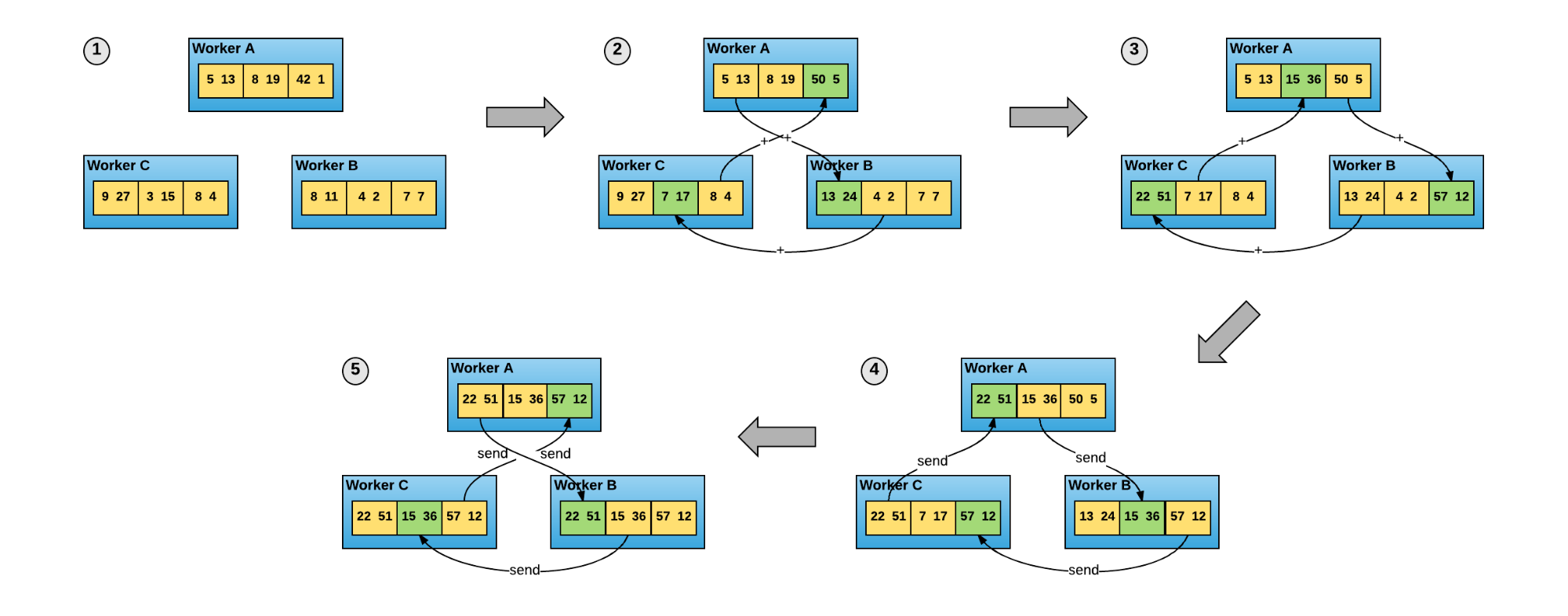
Ring-allreduce
The conventional data-parallel distributed training paradigm comprises 4 steps:
- Step 1: Each worker run a copy of training script and a portion of data. They will compute their local gradient.
- Step 2: The workers send their own gradient to the parameter-servers in order to combine the gradients.
- Step 3: The workers receive the combined gradient from the parameter-servers to update the model in each.
- Step 4: Repeat step 1.
There are some issues we must face when leveraging this paradigm:
- Decide the right ratio of workers to parameter-servers.
- It relates many components like clusters, workers, parameter-servers, etc…
In the early 2017, Baidu published his paper Bringing HPC Techniques to Deep Learning
as an effort to replace the above step 2 and step 3 using a protocol called ring-allreduce. In this paradigm, there is no parameter-servers to combine the gradient. The workers communicate with each other.
Consider that there are N nodes in the network, each worker will communicate 2*(N-1) times with the others. In the first (N-1) iteration, the gradients in the buffer are summed in the ring network fashion. In the second (N-1) iteration, we replace the gradient in all the node by the new one. Give the sufficient buffer, this paradigm can leverage the hardware capacity. Baidu suggest that this is the most bandwidth-optimal method until now. Furthermore, this method is more intuitive than the standard one. The all-reduce method can be found in MPI’s implementation like OpenMPI. The users just have to modify their programs of averaging the gradient using allreduce operation.
Introducing Horovod
Based on the previous observation, Uber has made several experiments and finally publish their stand-alone Python package named Horovod. In Horovod, Baidu ring-allreduce implementation is replaced by NCCL by NVIDIA. NCCL provides us a highly optimized ring-allreduce. In addition, NCCL 2 introduced the ability to run this operation across multiple machines in the network, which enables us to leverage the computation capacity of the distributed network. Not only that, Horovod could work with enormous models which resides on multiple GPUs while the original version can only support models fitting on a single GPU. Last but not least, the new API allows us to simplify our program much, as illustrated in the following.
def horovod_distributed_train(self):
    hvd.init()
    train_dir = os.path.join(self.train_cfg['train_dir'],
                                self.model_cfg['name'], 'train')

    cpkt_dir = os.path.join(self.common_cfg['log_root'],
                            self.model_cfg['name'], 'checkpoint')

    train_strategy = self.app.train_strategy(self.config, self.app)

    with train_strategy.graph_def, train_strategy.cpu_device:
        train_op = train_strategy.build_train_op()
        model = train_strategy.get_model_instance()
        self.app.build_graph_callback(model, train_op)

        param_stats = tf.profiler.profile(graph=tf.get_default_graph(),
                                            options=option_builder.ProfileOptionBuilder.trainable_variables_parameter())

        sys.stdout.write('Total params:%d\n' % param_stats.total_parameters)
        summary_hook = tf.train.SummarySaverHook(
            save_steps=self.train_cfg['save_steps'],
            output_dir=train_dir,
            summary_op=tf.summary.merge([model.summary(), ])
        )

        restoring_saver = tf.train.Saver(
            var_list=train_strategy.get_restoring_variables(
                self.train_cfg['restoring_global_step']),
            max_to_keep=self.train_cfg['max_to_keep'])
        training_saver = tf.train.Saver(
            var_list=train_strategy.get_saving_variables(
                self.train_cfg['saving_global_step']),
            max_to_keep=self.train_cfg['max_to_keep'])
        checkpoint_hook = tf.train.CheckpointSaverHook(
            cpkt_dir,
            save_steps=self.train_cfg['save_steps'], saver=training_saver,
            checkpoint_basename=model.__class__.__name__ + ".cpkt")

        logger_hook = self._create_logger_hook(train_strategy)
        app_stop_hook = self._create_stop_by_app_hook()

        config = tf.ConfigProto(allow_soft_placement=True,
                                log_device_placement=self.train_cfg['log_device_placement'])

        config.gpu_options.allow_growth = True
        config.gpu_options.visible_device_list = str(hvd.local_rank())
        hooks = [hvd.BroadcastGlobalVariablesHook(0),
                    tf.train.StopAtStepHook(last_step=self.train_cfg['max_steps'] // hvd.size()),
                    app_stop_hook,
                    logger_hook]
        if hvd.rank() == 0:
            hooks.append(checkpoint_hook)
            # NOTE: If the machine is the main worker, we will assign that checkpoint_hook
            # task to him

        with tf.train.MonitoredTrainingSession(
                hooks=hooks,
                chief_only_hooks=[summary_hook],
                save_summaries_steps=0,
                config=config) as mon_sess:

            if self.train_cfg['restore_sess']:
                print("Restoring saved session...")
                self._restore_session(restoring_saver, mon_sess,
                                        self.train_cfg['restore_checkpoint_path'],
                                        cpkt_dir)

            if hasattr(self.app, 'session_start_callback'):
                self.app.session_start_callback(mon_sess, model)

            dataset_loading_time = self.train_cfg.get('dataset_loading_time', 3)
            print("Delay %ds for starting queue runners." % dataset_loading_time)
            time.sleep(dataset_loading_time)
            while not mon_sess.should_stop():
                mon_sess.run(train_op)

        if hasattr(self.app, 'session_stop_callback'):
            self.app.session_stop_callback()
In the above code, there are some lines worth noticing:
- hvd.init() initializes Horovod.
- config.gpu_options.visible_device_list = str(hvd.local_rank) assigns a GPU to each of processes. Why local_rank ? Since the script run on a single machine with (possibly) multiple GPUs.
- opt=hvd.DistributedOptimizer(opt) wraps the TensorFlow optimizer, which provides the ability to use ring-allreduce.
- hvd.BroadcastGlobalVariablesHook(0) helps to broadcast the variables initialized by the first process to all other processes to ensure consistent initialization.
- I divide the max_step by the number of GPUs as max_step in my subconsciousness as well as in the configuration file is for a single GPU training, so in multiple GPUs training, we should divide the max_step by the number of GPUs.
Tensor Fusion
Recall that Give the sufficient buffer, this paradigm can leverage the hardware capacity, it means that this technique can perform best only if the tensors are large enough. In case of small tensors, we may fuse them first before performing ring-allreduce on them. To do this, Horovod establishes a secondary buffer and selects some small tensors to fit the fusion buffer. Obviously, the ring-allreduce operation is performed on the fusion buffer only.
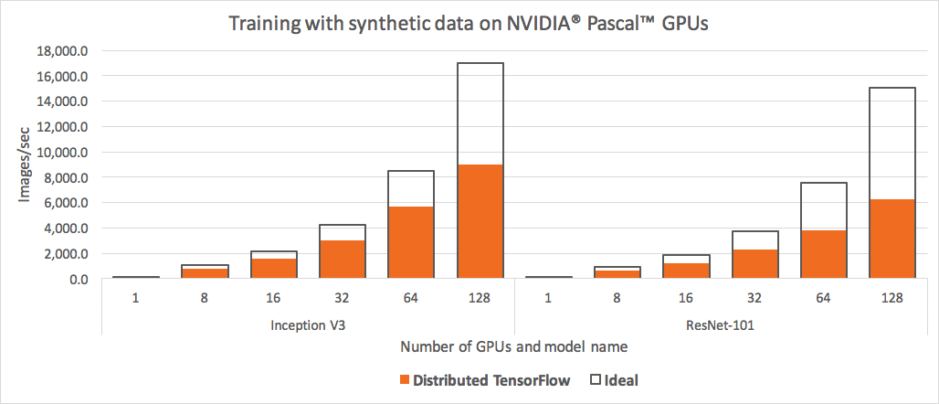
Horovod benchmark
The detail benchmark can be found in the Uber Engineering site. To be short, Horovod overpowers the traditional paradigm, especially when the number of GPUs grows higher.
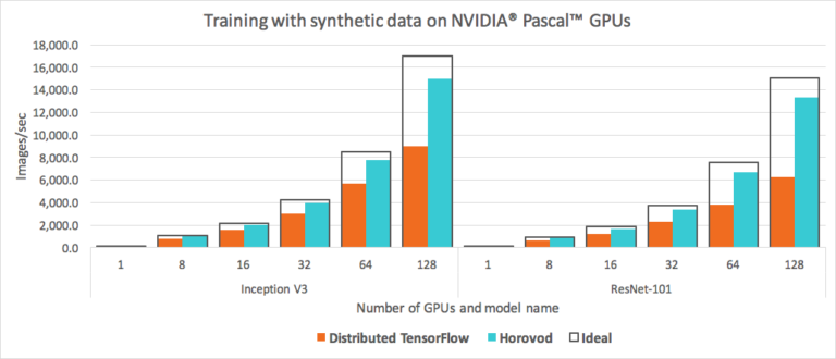
Uber also make a comparison between 2 communication protocols TCP and RDMI. However, we won’t discuss about it in this blog. You could read about it in the original blog of Uber.
Conclusion
To sum up, Facebook’s paper and Uber framework really make an echo in the community. They provide us a way to leverage distributing computing, which is important in the production. Horovod is still in its early stage of development, there are still some issues with it like MPI installation and deep learning scaling. In OtoNhanh.vn, we have implemented Horovod in our classification training and the result is promising, especially when people use the Amazon platform which allows the GPUs to be fully connected to each other.