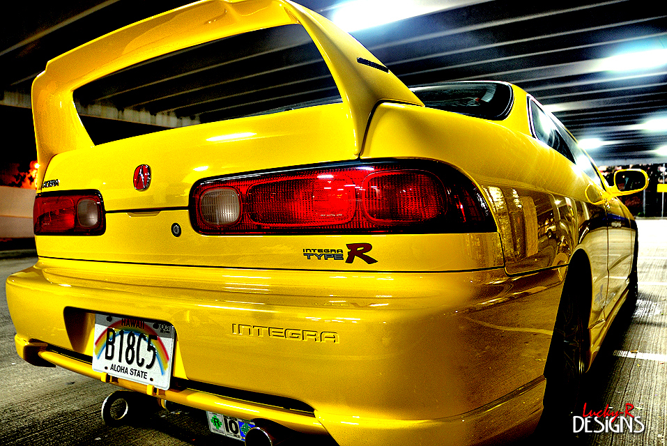
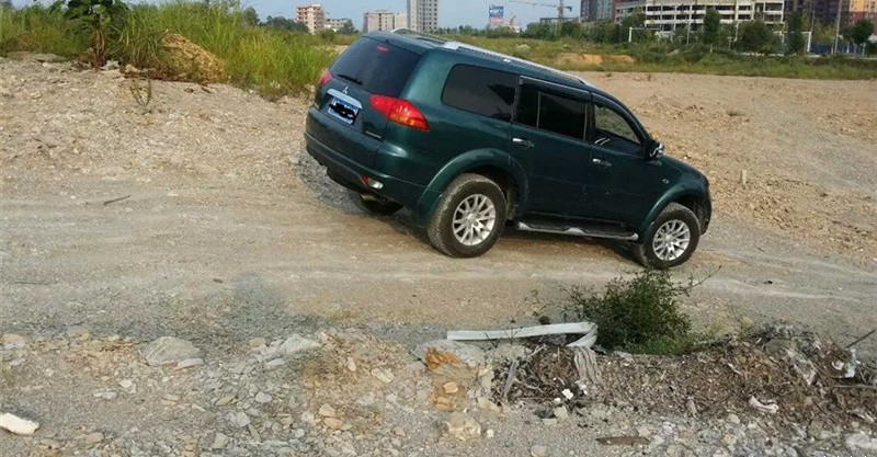
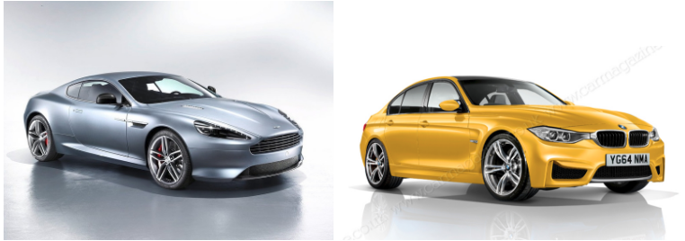
In OtoNhanh.vn, there is a section which allows the users to compare one model versus another in the aspect of specifications and the exterior as well as interior views. Normally, we will grab randomly 2 images of 2 models from the same category. Nevertheless, we observe that this approach doesn’t work well: Some images, in spite of belonging to the same category, cannot be compared to each other since the viewpoint, the pose, the scale of the car in the images, etc. are not matching. The origin of this disagreement is about the difference between semantic representation and visual representation. Therefore, we come up with the idea of establishing an indicator to compare the visual similarity between two images. In this blog, we will present our work towards that target.

I) K-Means Clustering
Considering that we work with the images of \((\sqrt{d},\sqrt{d}\)), so each image will be a point in the \(R_d\) space, K-Means will help to assign the similar points into the same cluster. How to define similar images? We will compute the Euclidean distance in the \(R_d\) space for example. Each above cluster will be represented by its centroid.

K-Means Clustering is a very well-known approach in unsupervised learning of Machine Learning (not Deep Learning!!!). It may be redundant to introduce this algorithm since it exists in every textbooks of Machine Learning. However, we still choose to introduce it briefly one more time with a simple implementation in Python.
Suppose we work with a data set \(\{x_1, x_2, ..., x_N\}\) in a \(R_d\) space. We want to gather the whole data set into K of clusters. In more detailed, each point in the data set will be partitioned based on its Euclidean distances with others. Each cluster will be represented by its centroid \(\mu_k\), \(k \in \{1,.., K\}, \mu_k \in R_d\). After the training, if we want to classify the new sample, we just need to assign it to the group with the nearest cluster to the sample. Pretty intuitive, yeah? Suppose hyperparameter K is known, the goal of the learning phase is to find the coordinates of the centroids and the assignment of each point.
To do this, we might want to add a variable to describe the assignment of data points to clusters. For each point \(x_n\), we introduce a corresponding variable \(r_{nk} \in \{0, 1\}\), where \(k = 1, ..., K\) describing which of K clusters the data point is assigned to. \(r_{nk} = 1\) means \(x_n\) belongs to cluster \(k\) and vice-versa. With this variable, we can define a loss function:
\[J = \sum_{n=1}^{N} \sum_{k=1}^{K} r_{nk} \|x_n - \mu_j\|^2\]To minimize this loss function, we use EM algorithm. In this approach, we initialize some valuea of \(\mu_k\), then in the first phase, we minimize the loss function w.r.t the binary \(r_{nk}\). In the second phase, we keep \(r_{nk}\) fixed and look for the value of \(\mu_k\) that makes \(J\) minimized. These two stages will alternate repeatedly until convergence. These two steps correspond respectively to the E(expectation) step and M(maximization) step of EM method.
This method belongs to a class of Mixture Model. Details of this model is beyond the scope of this blog, but you can read more in the Chapter 9 of Pattern Recognition and Machine Learning.
To be short, the formulas for these above steps are:
- E step:
- M step:
To build this algorithm from scratch is not easy, especially to the newbies. However, as this algorithm is too popular, we could find its API in many packets.
For example, this is a piece of code that we use K-Means in our application.
def get_dominant_colors(self, data, is_binary):
    img = self._get_image(data, is_binary)
    kmeans = KMeans(n_clusters=self.nbr_cluster).fit(img)
    label = kmeans.predict(img)
    unique, _ = np.unique(label, return_counts=True)
    dominant_label = unique[:self.nbr_dominant_color]
    return kmeans.cluster_centers_[dominant_label]
So we could find the centroids in d_dims space, then we could query two images from two models which belong to the same cluster for the comparison session. Nevertheless, this approach is not feasible: the training time is too long and we may end up training the model every time there are new images available.
II. Siamese Network and its variants
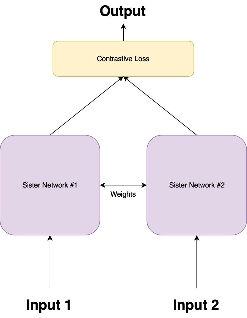
Siamese network is a special type of convolutional network. It is not used for classifying images, it is for learning the similarity between images. In this architecture, two images will be fed into two identical convolutional networks, then the two output will be inputs of a special loss function called Contrastive Loss Function for the purpose of differentiating two images. The ultimate goal of Siamese Network is to construct an embedding representation for the images in the form of vector. With the vectorized representation, we can use L2-distance or whatever other metrics to compute the similarity score between images.

In this section, we will focus on a variant of Siamese Network called Deep Ranking Model. We have finished building this model with TensorFlow and it will be used in OtoNhanh.vn soon.
In Deep Ranking, each sample consists of three images: anchor image, positive image which is akin to the anchor image and the negative image which is not in the same category with the anchor one. We call a group of three images like that a triplet.
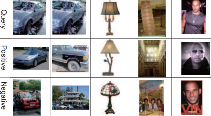
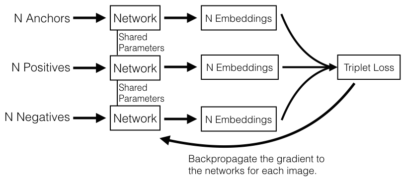
Three images will be again fed into three convolutional neural networks. The output will be given to a loss function called Triplet Loss Function to learn the similarities and the differences between the images.
Network Architecture
So what is the architecture of Deep Ranking model exactly?
According to the author:
We design a novel multi-scale deep neural network architecture that employs different levels of invariance at different scales.
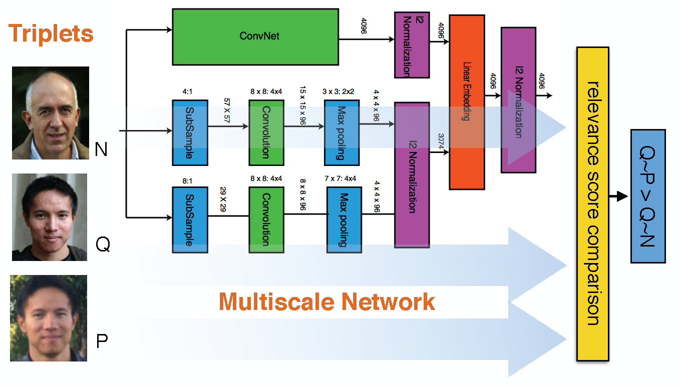
In this architecture, the ConvNet can be any kind of convolutional neural network, including AlexNet, VGG, etc… In our model, we employ ResNet because of its superiority. ConvNet plays the role of encoding strong invariance and capturing the image semantics. The other two shallower networks rather capture visual appearance. The outputs of these pipelines will be normalized and combined as an embedding.
Triplet Loss Function
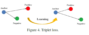
Thanks to convolutional network, we obtain a mapping \(f\) to transform images to vectors. Suppose that \((p_i, p_i^+, p_i^-)\) is a triplet. We hope that after the training, with the metric \(D\), we get:
\[D(f(p_i, p_i^+)) < D(f(p_i, p_i^-))\]To realize that target, the author suggest using Hinge Loss:
\(l(p_i, p_i^+, p_i^-) = max\{0, g + D(f(p_i, p_i^+)) - D(f(p_i, p_i^-))\}\)
Minimizing this loss function encourages the distance between the \((p_i, p_i^+)\) is less that between \((p_i, p_i^+)\) by a value of \(g\).
Triplet Sampling
As we can see, the intuition of network architecture and loss function is not complicated. Nonetheless, the real challenge of this model is how to sampling the triplet effectively? We cannot choose the too easy triplet: this make the training easily over-fitted. In the original paper, the author introduced an additional metric \(r\) to measure the similarity between images: As the training goes further, we will insert a triplet with the furthest positive image and nearest negative image to regularize the training. However, he didn’t clarify the metric \(r\). So we have to find another way to get around it.
In the paper In Defense of the Triplet Loss for Person Re-Identification, the authors suggested using the same metric \(D\) for the triplet sampling during the training. This method is called Batch Hard. Supposing in the mini-batch \(X\), we have \(P\) classes and there are \(K\) images in each class. Images from the same class can be paired positively and vice-versa. This raises another challenge in term of batch sampling: How to sample a batch with at least three classes with at least 2 images in each class?
\[L_{BH}(f, X) = \overbrace{\sum_{i=1}^{P}\sum_{a=1}^{K}}^{\text{all anchor}} max(0, g + \overbrace{\max_{p=1..K} D(f(x_a^i), f(x_p^i))}^{\text{hardest positive}} - \overbrace{\min_{j=1..P,\\ n=1..K, \\j \neq i} D(f(x_a^i), f(x_n^i))}^{\text{hardest negative}})\]However, we argue that we may have to pay the price of slower training in order to realize the selection of triplet during the training. So we may want to select the triplets first by ourselves for the faster training.
Implementation
In our implementation, we’ve done some modifications:
-
We pass the anchor image, positive image and negative image successively to a single pipeline to construct their embedding representations instead of three identical networks to save memory while training on GPUs.
-
We will define the triplets manually or by boot-straping before training and write the triplet path to a text file.
-
In the original paper, they employed 4000-dims embedding vector. However, we observe that during our training 128-dims vector outperforms 4000-dims one. This is super queer to us as it seems intuitive that vector with bigger dimension must capture more features. This issue will be investigated carefully during our deployment.
Source code for model network:
def _build_conv_net(self, images, config, depths, res_func, name='resnet'):
    """
    Construct embedded representation for images using ResNet
    :param images: input of the network
    :param config: configuration file
    :param depth: depth of ResNet
    :param res_func: sub-function used in ResNet
    :param name: variable_scope
    :return:
        Embedded representation of image
    """
    with tf.variable_scope('first_pipeline'):
        first_output = _build_resnet(images=images, config=config,
                                    depths=depths, res_func=res_func,
                                    name=name)
        first_output = tf.nn.l2_normalize(first_output, axis=1)
        mean = tf.reduce_mean(first_output, axis=1)
        mean = tf.expand_dims(mean, axis=1)
        first_output = tf.subtract(first_output, mean)

    with tf.variable_scope('second_pipeline'):
        second_output = slim.conv2d(inputs=images, num_outputs=32,
                                    kernel_size=8, stride=32, padding='SAME')
        second_output = slim.max_pool2d(second_output, kernel_size=7, stride=5,
                                        padding='SAME')
        second_output = slim.flatten(second_output)
        second_output = tf.nn.l2_normalize(second_output, axis=1)
        mean = tf.reduce_mean(second_output, axis=1)
        mean = tf.expand_dims(mean, axis=1)
        second_output = tf.subtract(second_output, mean)

    with tf.variable_scope('third_pipeline'):
        third_output = slim.conv2d(inputs=images, num_outputs=32,
                                kernel_size=8, stride=48,
                                padding='SAME')
        third_output = slim.max_pool2d(third_output, kernel_size=5, stride=8,
                                    padding='SAME')
        third_output = slim.flatten(third_output)
        third_output = tf.nn.l2_normalize(third_output, axis=1)
        mean = tf.reduce_mean(third_output, axis=1)
        mean = tf.expand_dims(mean, axis=1)
        third_output = tf.subtract(third_output, mean)

    merge_one = tf.concat([second_output, third_output], axis=1)
    if merge_one.get_shape()[1] != first_output.get_shape()[1]:
        merge_one = slim.fully_connected(inputs=merge_one,
                                        num_outputs=int(first_output.get_shape()[1]),
                                        activation_fn=None)
    merge_two = merge_one + first_output
    return merge_two
Source code for triplet loss function:
def _calc_triplet_loss(self, a_embedding, p_embedding, n_embedding, margin, epsilon=1e-7):
    """
    Calculate the triplet loss
    :param a_embedding: anchor image of the triplet
    :param p_embedding: image from the same class with the anchor image (positive)
    :param n_embedding: image from the different class with anchor image (negative)
    :param margin: margin value between the distances
    :param epsilon: the value used in tf.clip_by_value
    :return:
    """
    a_embedding = tf.clip_by_value(a_embedding, epsilon, 1.0 - epsilon)
    p_embedding = tf.clip_by_value(p_embedding, epsilon, 1.0 - epsilon)
    n_embedding = tf.clip_by_value(n_embedding, epsilon, 1.0 - epsilon)
    margin = tf.constant(margin, shape=[1], dtype=tf.float32)
    pos_dist = tf.reduce_sum(tf.square(tf.subtract(a_embedding, p_embedding)), axis=1)
    neg_dist = tf.reduce_sum(tf.square(tf.subtract(a_embedding, n_embedding)), axis=1)
    basic_loss = tf.add(tf.subtract(pos_dist, neg_dist), margin)
    return tf.reduce_mean(tf.maximum(basic_loss, 0.0), 0)
Results
We are still in the first phase of deploying this model into production. However, the result is very promising: This model can produce a very high margin between the positive pair and negative pair:

In the future, we have an intention to improve the triplet sampling during the training. It is anyway the optimal approach to improve the ability of differentiating the images.