Clustering and Retrieval (Part 1)

At the moment, we are working in a big project of personalized news distribution for 24h News. In this project, we assume that each reader of this page has their own taste, so we can’t deliver the same content to them: we have to explore their favorite and then deliver news based on that observation. However, at the production scale, suppose we have millions of clients, the generation of millions of different content seems extreme expensive. So we have the idea of clustering our customers into N clusters, then generate N different contents for the cluster centroids. This idea seems plausible to us. In this blog, I want to tell you about the journey of finding the best clustering algorithm.

I. What is retrieval and what is clustering

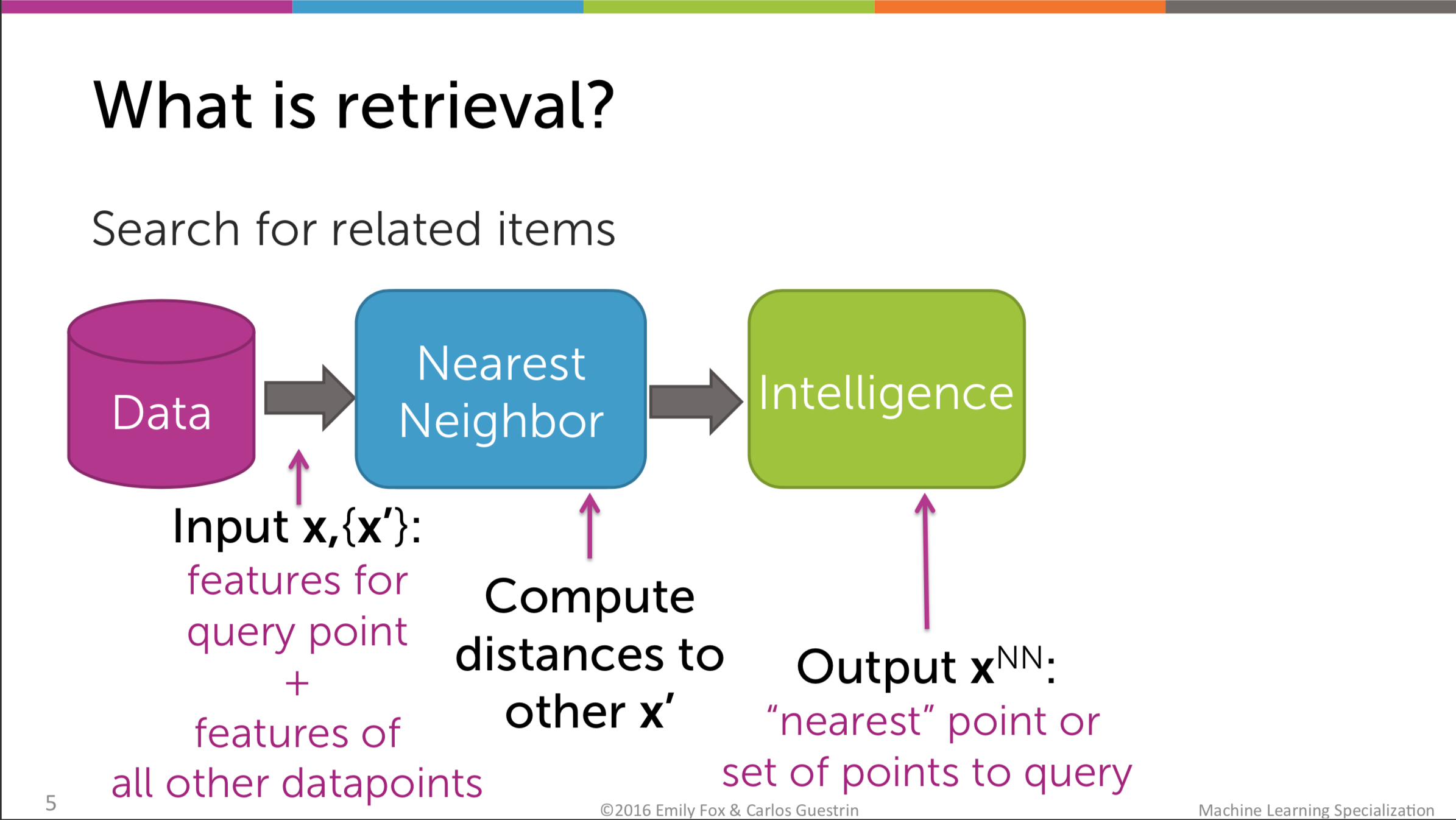
Giving an item, retrieval helps you to find a similar item to that by calculating the distances between the given item and every other items in the item space. To do this, the most important task is to find an appropriate metrics which helps you to compute the similarity between things.

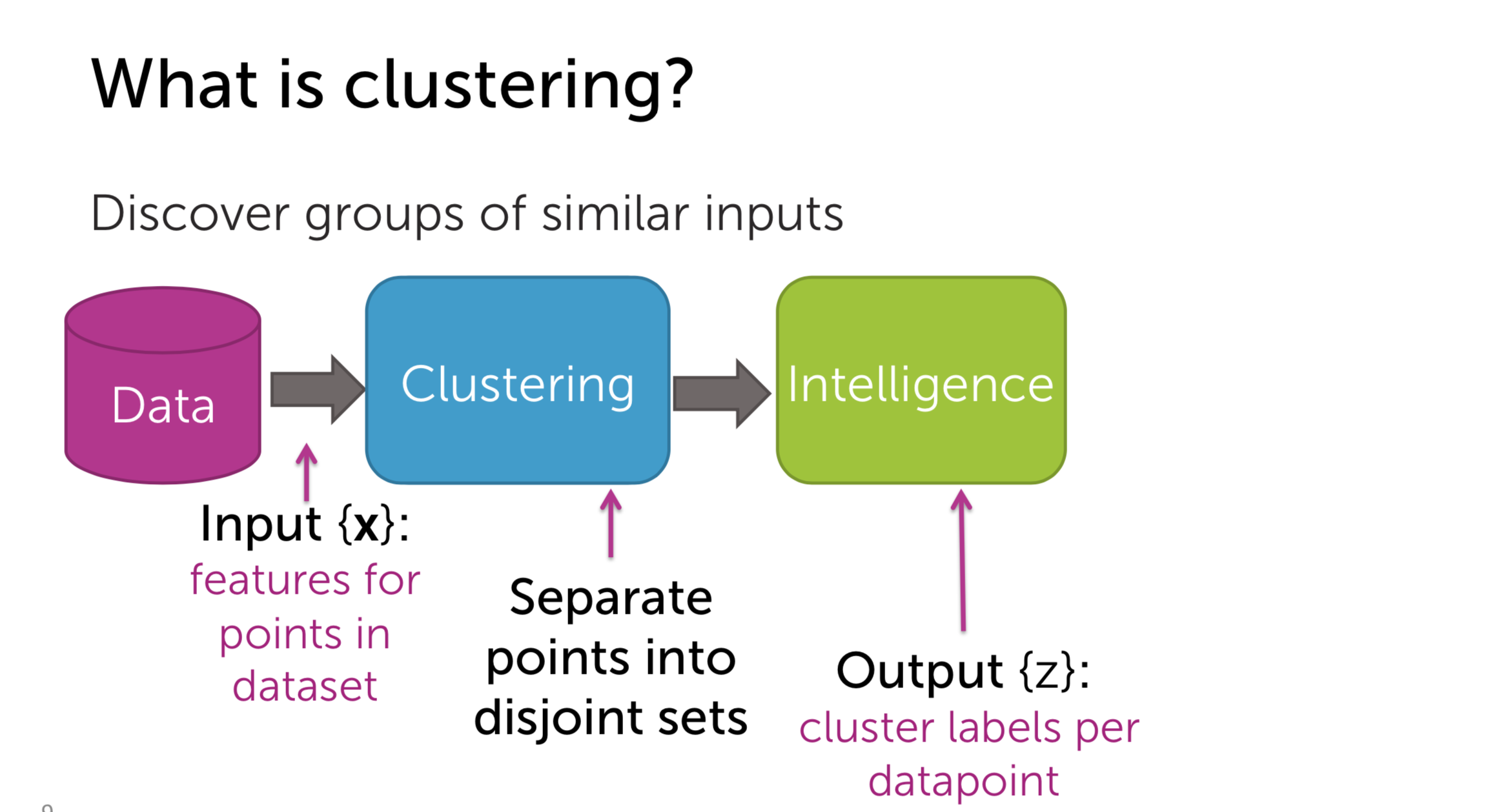
On the other hand, clustering helps you to group the similar items in the space. Items with similar characteristics will be near each other and then we assume that they are in the same cluster. Obviously, every problem which is related to similarity is in need of a distance metrics. Each cluster will be represented by its centroid, which is in most cases the average point of the items in that cluster.

II. Nearest Neighbor Search

Nearest Neighbor Search is the very symbolic technique of Retrieval method. In this approach, we compute the distance between the anchor and the other items in the space. For example, you are reading an article and you want to read the similar articles. Every articles will be represented by vector. Then we compute the distance, maybe with L2-distance so we can get the article with the minimum distance.

There are two types: query the most similar item (1-NN algorithm) and query the most k similar items (k-NN algorithm):

1-NN algorithm

The idea is pretty simple, just like what I said above

• Pseudo-code:

Initialize Dist2NN = $$\infty$$
For i = 1, 2, .., N:
    compute $$\delta$$ = distance($$x, x_i$$)
    if $$\delta$$ < Dist2NN:
        Dist2NN = $$\delta$$

return the item with distance Dist2NN

k-NN algorithm

In this algorithm, we keep the record of most k similar items.

• Pseudo-code:

Initialize Dist2kNN = sorted($$\delta_1, \delta_2, .., \delta_k$$)

for i = k+1, .., N:
    $$delta_i$$ = distance($$x, x_i$$)
    if $$\delta_i$$ < Dist2kNN[k]:
        insert $$\delta_i$$ into the sorted list Dist2kNN

return the items with the distance in Dist2kNN

The idea of the algorithm is really simple and intuitive, however, to guarantee the efficiency of the algorithms, there are 2 critical elements that need considering carefully: the vectorized representation of items and distance metrics.

Vectorization

In case of text, there are many methods that could help us to vectorize the documents, like:

• Bag of Word (BoW): It is quite similar to the histogram in the visual domain. We count the occurrence of each word in the corpus, then make the vector with that. There is a major drawback with this idea: There are some words which appear in almost every document like a, the, you, etc.

• TF-IDF: It uses the same idea of word count, but TF-IDF penalize the score of words which appear in different documents in the corpus. Differently speaking, it favors the locally common words but disfavors the globally common words. TF stands for Term Frequency, IDF stands for Inverse Document Frequency. Details about this approach can be found easily from the Internet.

Distance metrics

• Scaled Euclidean Distance

\(a_1, .., a_d\) are the weights for each feature. This feature selection is in fact not very popular in reality since feature engineering is always hard for us. So the non-scaled version is more preferable:

• Cosine similarity

There are many other metrics, for example: Manhattan, Jaccard, Hamming, etc.

Complexity of algorithms

As you can see, for each query, we have to sweep through the whole data-set, so it is really computationally demanding. The complexity for 1-NN and k-NN is \(O(N), O(Nlog(k))\) respectively. This level of complexity is really infeasible in real life applications. So we have to improve it.

KD-tree

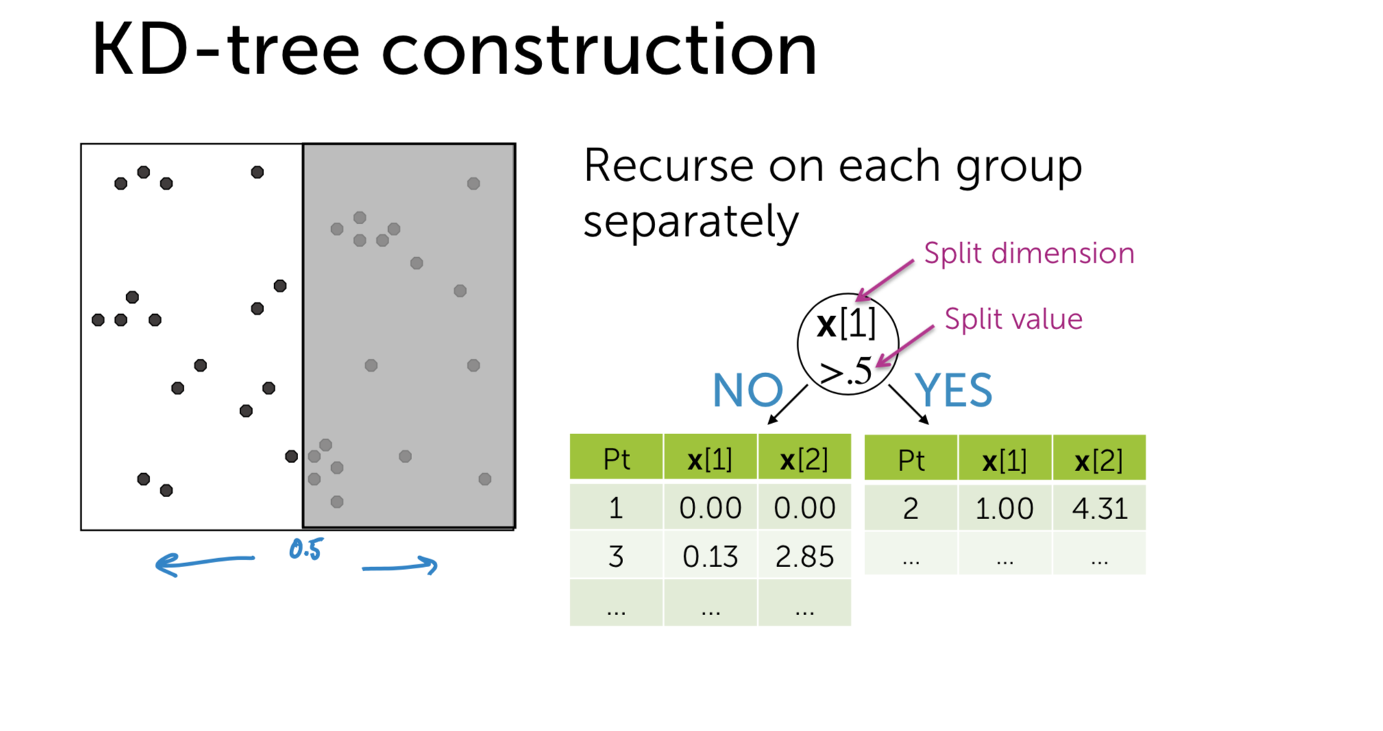
We could divide the item space into the binary tree with respect to its features:

So, as you can see, I use a Tree data structure to accelerate query time. And now, how to implement it in our problem of Nearest Neighbor?

There are three steps:

• Step 1: Exploring the leaf node that contains our query item:

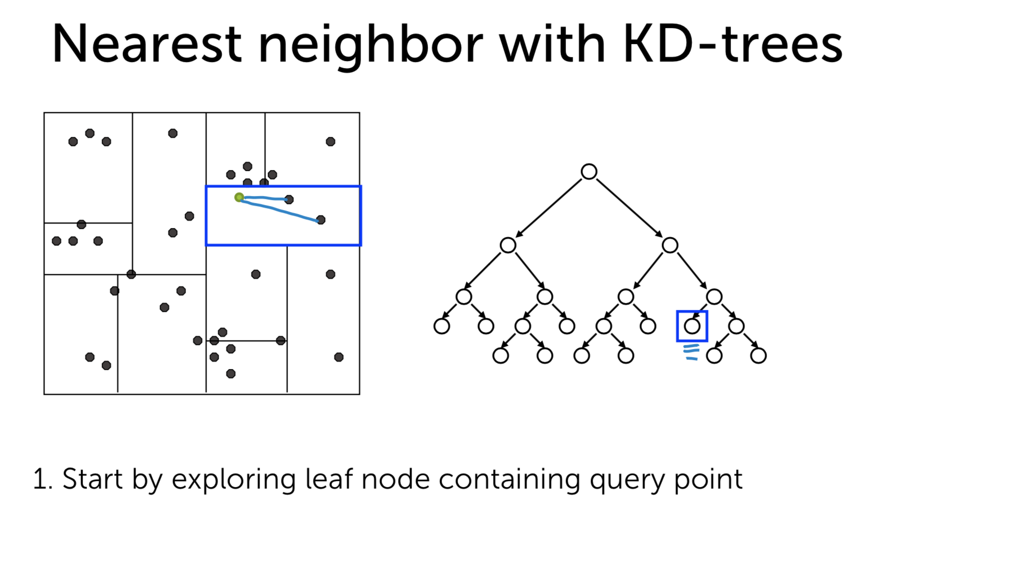
• Step 2: Compute the distance to other points in the leaf node and save the nearest distance to \(NN\)

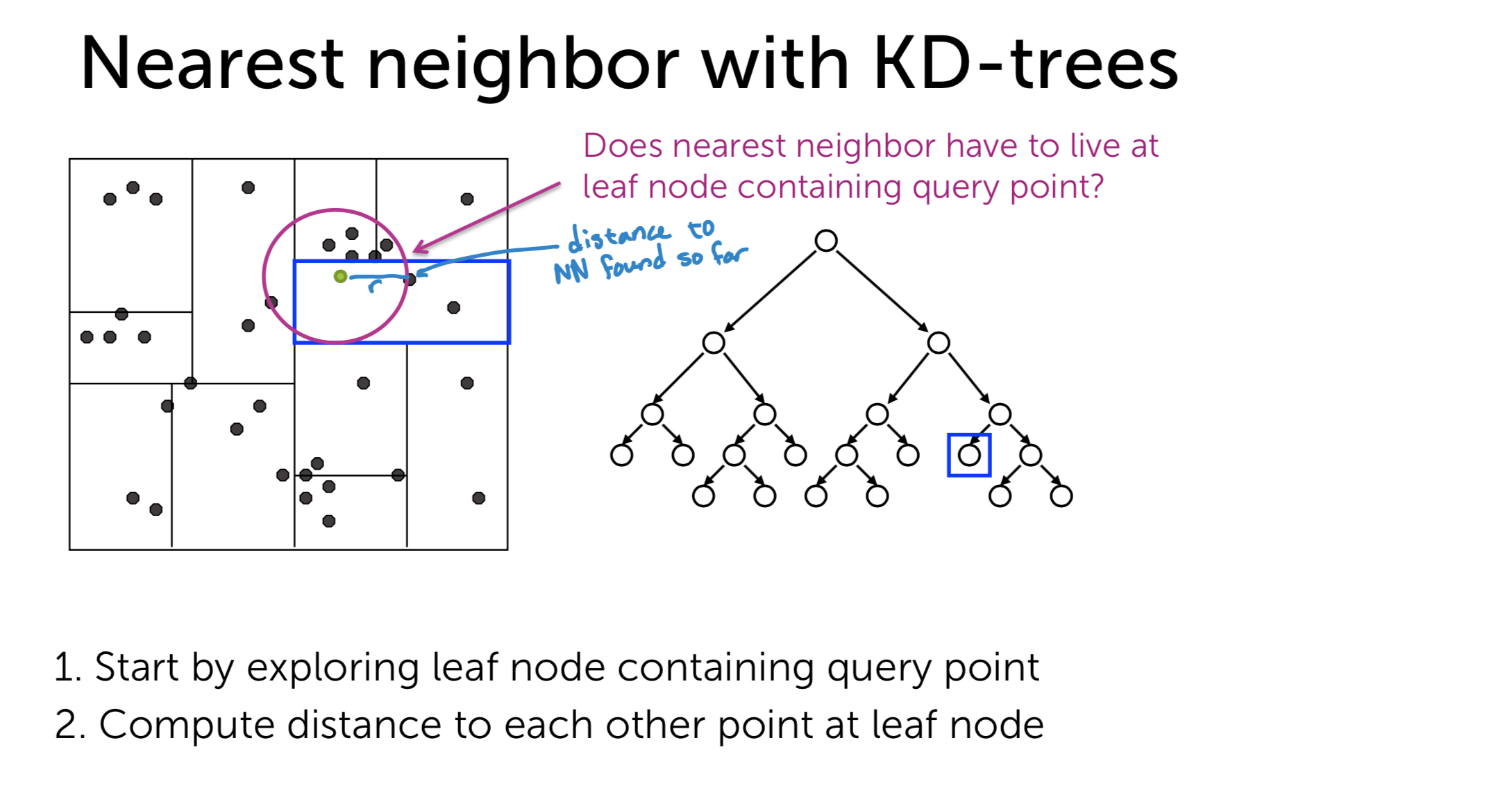
• Step 3: Backtrack using traversal technique and try other branches. If the distance from the query point to the branch is shorter than the current nearest distance, we examine this branch to compute the (maybe) next nearest distance. If not, we just ignore the branch and move the next one.

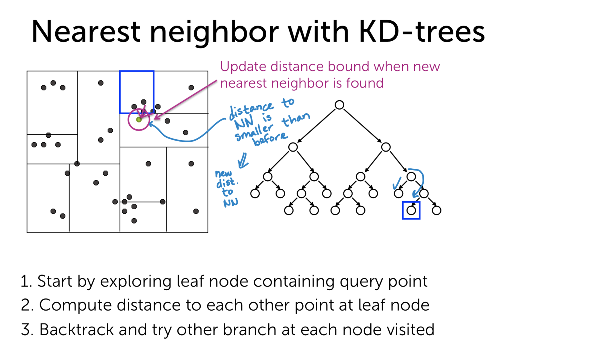
The worst-case complexity of this approach for 1-NN is \(O(N)\) and for k-NN is \(O(N^2)\). However, the worst-case is really rare, so we could save a lot of resources using this techniques. We can also use pruning to approximate this technique. Instead of ignoring the branch if the distance to it is longer than \(NN\), we can ignore it if it is longer than \(NN/\alpha\) (\(\alpha > 1\)).

Local sensitive hashing

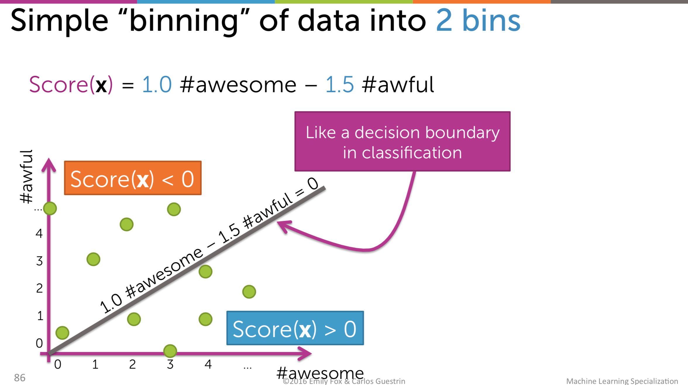
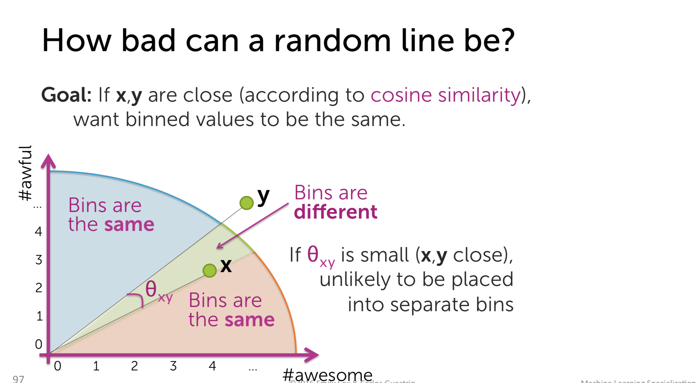
KD-Tree is cool but it has its own drawbacks. First of all, it is not easy to implement it efficiently. Secondly, when the dimension of the vector is large, the computation is quite expensive. So we move to another method: Local sensitive hashing. In this method, we define the line to divide the item space into different bins and we just examine the items residing in the same bin with the query one.

Surely, when binning like this, there will be cases that we cannot find the nearest neighbor:

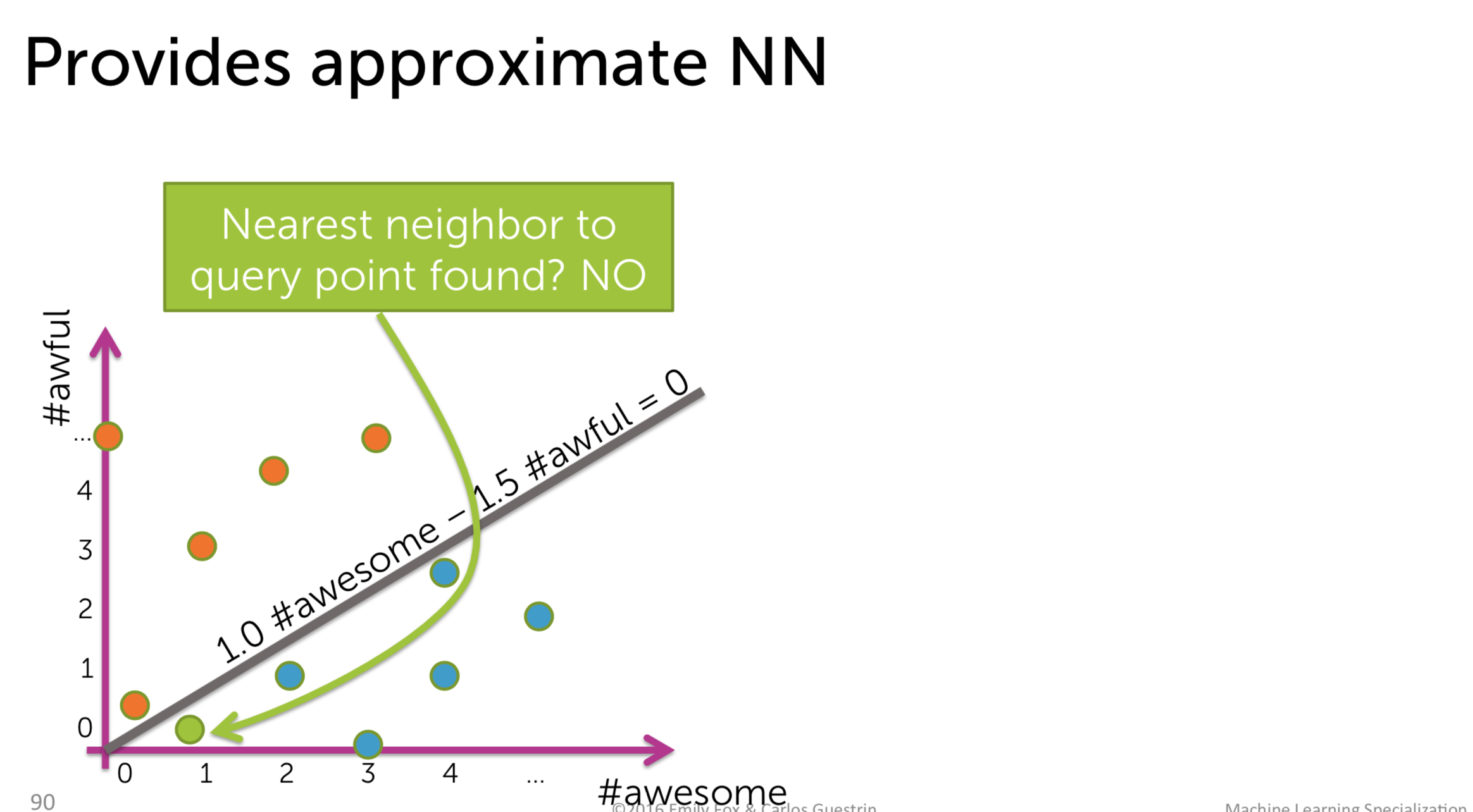
So, the question here is, how to do the binning efficiently? The answer is simple: leave it to the fate, just do the binning randomly. The probability that two similar points reside in different bins is small.

Furthermore, we could reduce the searching cost by using more bins, even though we risk to have the nearest neighbor in the different bin. It is a trade-off that we have to accept.

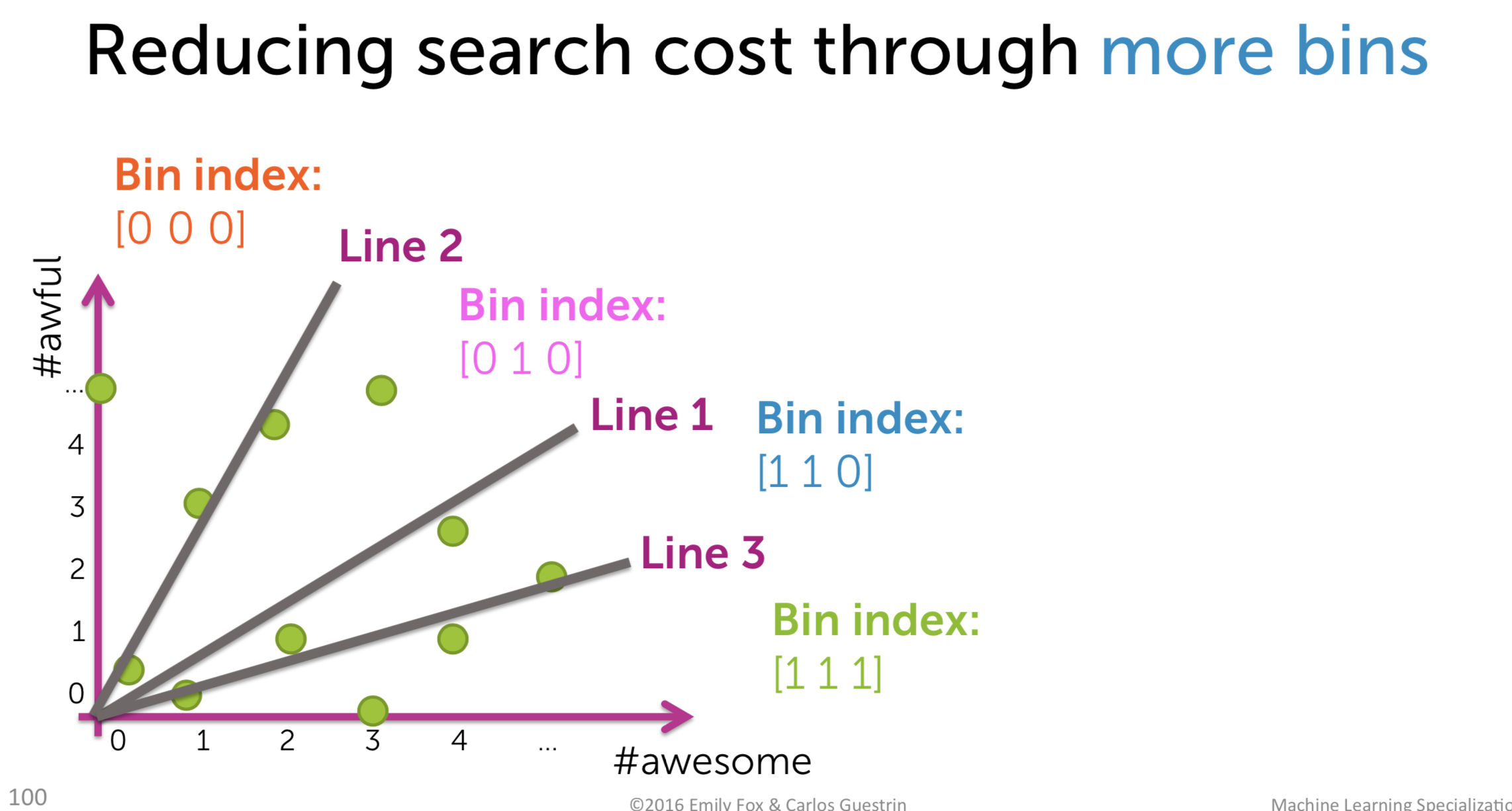
To sum up, to realize this method, we do the following steps:

• Draw \(h\) line randomly

• Compute score for each bin and translate to binary index, use the collection of binary index as bin index

• Create a hash table

• Search the bin in which the query one stays, and if possible, examine the neighboring bins

III. Reference

• Machine Learning: Clustering & Retrieval