In the age when vision technology thrive remarkably, Computer Vision and its application become more and more rife, particularly in retail industry where a host of issues remains unsolved. In AWL Vietnam, we are concentrating on developing a system detecting wrongdoings and analyzing customers’s behaviours. One of the concrete pillar of this system is the module of Pose Extraction.
I. Overview
There are two approaches to solve this problem: top-down and bottom-up. In top-down approach, we detect the keypoints of one person in the image while the bottom-up, the model is capable of detecting the pose of several people in the image. Each has its own perks:
-
Top-down method: In case of multi-people case, we need to employ the human detection model to explore all the bounding boxes containing person. So in this case, the processing time is proportional to the number of people is this frame. However, this model is accurate as it can resolve the occlusion and overlapping in many cases.
-
Bottom-up method: This model could detect the joints of many people at once. In order to connect joints from different people, this architecture also predicts joints connection. Even though this method guarantees stable speed during inference, its performance in term of accuracy is poor.
II. Top-down approach
A representative architecture of this method is HourGlass. This network design is motivated by the need of coherent understanding of body and scale invariance. This architecture consists of two main elements: backbone block and refinement blocks:
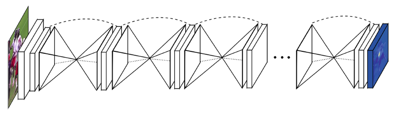
In HourGlass, backbone resembles ResNet architecture much and this module is used to predict the very first output, which is heatmaps in the context of pose estimation, each heatmap for each joint. Hourglass-like refinement blocks receive this prediction as a starting point. They execute consecutively several down-sampling and up-sampling layers to produce more refined heatmaps. The more the number of refinement blocks, the better the final results seem to be.
Forward flow looks like this:
def forward(self, x):
    # x [N*256*256*3]
    out = []
    x = self.conv1(x)
    x = self.bn1(x)
    x = self.relu(x)

    x = self.layer1(x)
    x = self.maxpool(x)
    x = self.layer2(x)
    x = self.layer3(x)
    # x [N, 64, 64, num_joints]

    for i in range(self.num_stacks):
        y = self.hg[i](x)
        y = self.res[i](y)
        y = self.fc[i](y)
        score = self.score[i](y)
        out.append(score)
        if i < self.num_stacks-1:
            fc_ = self.fc_[i](y)
            score_ = self.score_[i](score)
            x = x + fc_ + score_
    # out [num_stacks, N, 64, 64, num_joints]
    return out
Intermediate Supervision
Another interesting point of HourGlass implementation is that the final loss is computed from heatmaps of every refinement block. This guarantees better prediction after every refinement blocks, not only the last one.
loss = 0
for o in output:
    loss += criterion(o, target, target_weight)
Knowledge distillation
Thanks to this stacked architecture, we are able to use knowledge distillation technique. We could use model with more stacks to teach the less one which is more lightweight. However, in my experiments, improvement is limited when I trained student model using ground-truth labels and teacher model.
for j in range(0, len(output)):
    _output = output[j]
    kd_loss += criterion(_output, t_output, target_weight)
    gt_loss += criterion(_output, target, target_weight)
acc = accuracy(score_map, target, idxs=idxs)
# This is confirmed from the source code of the authors. This is weighted sum of loss from each heat-map
total_loss = kdloss_alpha * kd_loss + (1.0 - kdloss_alpha) * gt_loss
Data Preparation and Loss Function
For each bounding box, we have corresponding joint coordinates. In order to transform these numbers into useful labels. We use Gaussian Transform to create heatmaps from coordinates:
def generate_target(self, joints, joints_vis):
    '''
    :param joints:  [num_joints, 3]
    :param joints_vis: [num_joints, 3]
    :return: target, target_weight(1: visible, 0: invisible)
    '''
    target_weight = np.ones((self.num_joints, 1), dtype=np.float32)
    target_weight[:, 0] = joints_vis[:, 0]

    assert self.target_type == 'Gaussian', \
        'Only support gaussian map now!'

    target = np.zeros((self.num_joints,
                       self.heatmap_size[1],
                       self.heatmap_size[0]),
                      dtype=np.float32)

    tmp_size = self.sigma * 3

    for joint_id in range(self.num_joints):
        feat_stride = self.image_size / self.heatmap_size
        mu_x = int(joints[joint_id][0] / feat_stride[0] + 0.5)
        mu_y = int(joints[joint_id][1] / feat_stride[1] + 0.5)
        # Check that any part of the gaussian is in-boundsG
        ul = [int(mu_x - tmp_size), int(mu_y - tmp_size)]
        br = [int(mu_x + tmp_size + 1), int(mu_y + tmp_size + 1)]
        if ul[0] >= self.heatmap_size[0] or ul[1] >= self.heatmap_size[1] \
                or br[0] < 0 or br[1] < 0:
            # If not, just return the image as is
            target_weight[joint_id] = 0
            continue

        # # Generate gaussian
        size = 2 * tmp_size + 1
        x = np.arange(0, size, 1, np.float32)
        y = x[:, np.newaxis]
        x0 = y0 = size // 2
        # The gaussian is not normalized, we want the center value to equal 1
        g = np.exp(- ((x - x0) ** 2 + (y - y0) ** 2) / (2 * self.sigma ** 2))

        # Usable gaussian range
        g_x = max(0, -ul[0]), min(br[0], self.heatmap_size[0]) - ul[0]
        g_y = max(0, -ul[1]), min(br[1], self.heatmap_size[1]) - ul[1]
        # Image range
        img_x = max(0, ul[0]), min(br[0], self.heatmap_size[0])
        img_y = max(0, ul[1]), min(br[1], self.heatmap_size[1])

        v = target_weight[joint_id]
        if v > 0.5:
            target[joint_id][img_y[0]:img_y[1], img_x[0]:img_x[1]] = \
                g[g_y[0]:g_y[1], g_x[0]:g_x[1]]

    return target, target_weight
Since both predictions and targets are continuous variables, we use MSELoss to compute the loss between those.
Pros and cons
It is undeniable that accuracy of this approach is higher in both public datasets (MPII, COCO) and private datasets. Nevertheless, its dependence on person detection poses several challenges for me. Firstly, overall speed relies heavily on the number of bounding boxes. The more this number is, the slower the whole system runs. Secondly, it also depends on the quality of bounding box. If person detection module fails to capture the whole body, top-down methods cannot deduce accurate keypoints.
III. Bottom-up approach
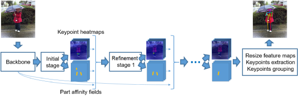
The most renowned architecture must be OpenPose by CMU. Generally speaking, this approach does not only predict heatmaps but also Part Affinity Field (PAF) which could be described as pairwise connection between keypoints. This extension helps us to differentiate keypoints from different people in the same frame. Bottom-up architecture shares the same iterative idea of top-down approach when the result is refined over and over in order to produce satisfactory result. It consists of two parts:
- ConvNet provides two tensors: keypoint heatmaps and their corresponding pairwise relations (PAFs).
- Grouping keypoints of same person to each other to acquire the initial prediction. This prediction will be refined over successive stages.
The original implementation is on Caffe and quite heavy. There has been tremendous effort to bring this architecture to mobile devices or embedded systems, Lightweight OpenPose is one of those. In this implementation, they use lightweight backbones like MobileNetV2 or ShuffleNet instead of VGG16. Furthermore, they leverage shared computation to accelerate inference speed. Having said that, from my observation, its accuracy is not high enough for real-life applications.
In Lightweight OpenPose, initial predictions of keypoints and PAFs are made like this:
class InitialStage(nn.Module):
    def __init__(self, num_channels, num_heatmaps, num_pafs):
        super().__init__()
        self.trunk = nn.Sequential(
            conv(num_channels, num_channels, bn=False),
            conv(num_channels, num_channels, bn=False),
            conv(num_channels, num_channels, bn=False)
        )
        self.heatmaps = nn.Sequential(
            conv(num_channels, 512, kernel_size=1, padding=0, bn=False),
            conv(512, num_heatmaps, kernel_size=1, padding=0, bn=False, relu=False)
        )
        self.pafs = nn.Sequential(
            conv(num_channels, 512, kernel_size=1, padding=0, bn=False),
            conv(512, num_pafs, kernel_size=1, padding=0, bn=False, relu=False)
        )

    def forward(self, x):
        trunk_features = self.trunk(x)
        heatmaps = self.heatmaps(trunk_features)
        pafs = self.pafs(trunk_features)
        return [heatmaps, pafs]
Furthermore, if you want to find out how they create PAFs label for training, please have a look at their original github repository.
Pros and cons
Advantages
- Inference speed stays stable during inference speed since its input is frame, not bounding box.
- It simplifies the whole system since we don’t have to integrate person detection module.
Disadvantages
- The unavailability of tracking module: Since we don’t have bounding boxes at our disposal, we cannot utilise traditional tracking algorithms like Sort or DeepSort. At the moment, there is a new efficient solution for this named Spatial Temporal Affinity Field, however implementation in popular frameworks is not available yet.
- Partial Estimation is not possible. In many cases, we don’t want to predict all the keypoints. However, the whole idea of bottom-up approach is to connect nearby keypoints so discrete inference is impossible; it requires a subset of connected keypoints to be workable.
- Accuracy is pretty low.
IV. Conclusion
Based on my experience, while recent improvement for top-down methods is negligible, there is a great deal of space for bottom-up approach to enhance, including accuracy and tracking ability. This is the issue that my team and I aim to tackle in the next stage.