In the previous blog, I have discussed YOLACT, a common instance segmentation architecture and my grudges against it and its variants. In this blog, I will introduce another architecture, which I believe a more efficient design. This is namely SOLO.
Before SOLO, the authors claim that there are two main paradigms to solve instance segmentation problems, like pose pose estimation, top-down and bottom-up. YOLACT falls into the former group when it tries detect-then-segment approach: it relies heavily on detection result to have a satisfactory mask representation. The latter tries to assign an embedding vector so that post-processing step could group these pixels into the same instance easily. Frankly speaking,
I haven’t figure out how the latter works, especially the classification step. Anyway, both approaches are step-wise, which basically mean slow performance and (maybe) poor accuracy. Nevertheless, none of this matters anyway since we have SOLO in our life.
I. SOLO
My first impression is that this architecture is inspired a lot from SSD. The whole image is split into nxn grids, each is responsible for detecting mask whose center lies in this grid cell. Furthermore, its backbone also generate a pyramid of feature maps with different sizes, each becomes an input for prediction heads: semantic classification and instance mask. Finally, NMS will be required to filter out highly-overlapped masks.
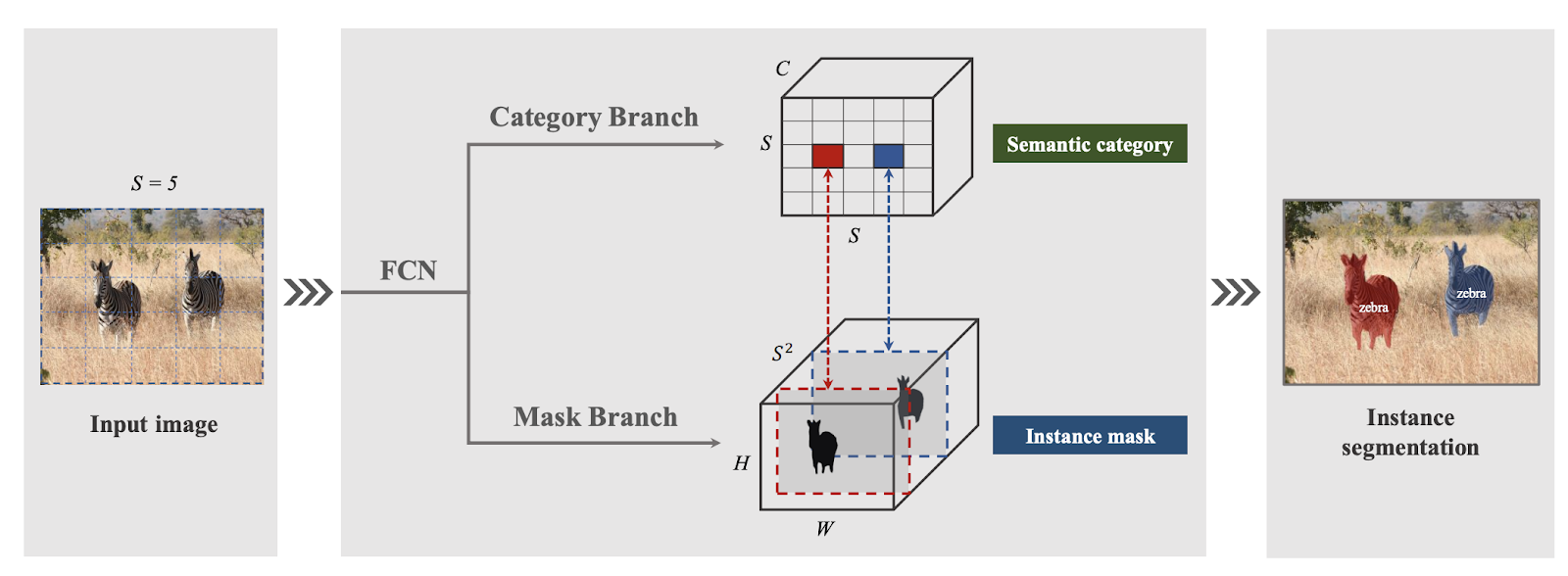
In more detailed, its backbone outputs several feature maps of different heights and widths but the same channels (
normally 256 channels). The first branch is tasked with classifying each grid with corresponding label. Therefore, it
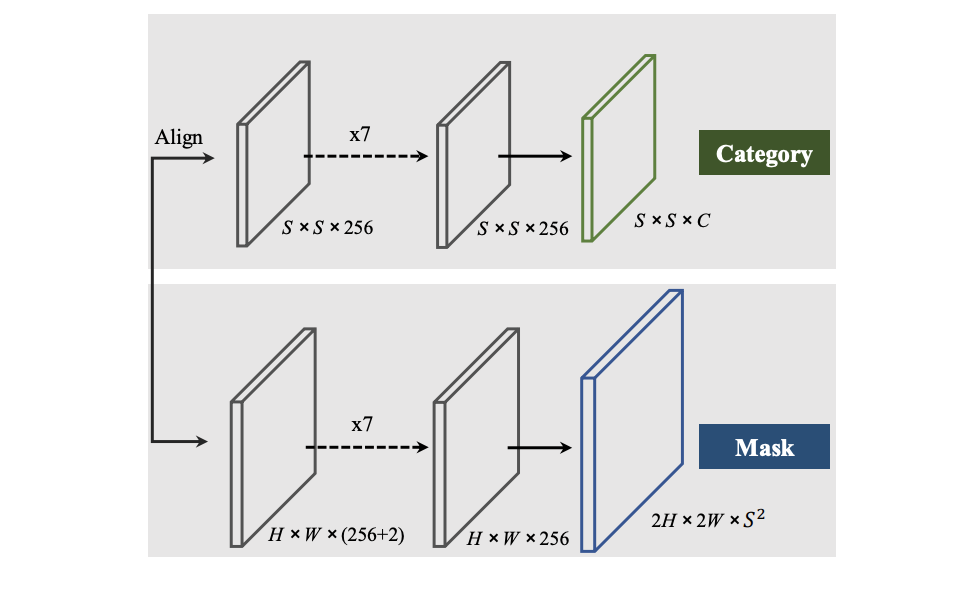
produces a tensor with shape SxSxC for each image. With this purpose in mind we have to align these feature maps to new size SxS, using pooling or interpolation. Afterward, several 1x1 convolutions are employed to create SxSxC
final category matrix.
On the other hand, the second branch has to produce a mask for each grid if this grid stays in the center of the predicted mask. Thus, the output of this branch is a tensor with WxHx(S*S). Similarly to object detection, this may
output numerous overlapped masks, therefore, it requires a NMS layer to do the post-processing. In this branch, it seems to be more direct when 1x1 convolutions are used to transform feature maps into wanted mask representations.
Please note that there are additional 2 channels in the following figure because CoordConv is used to improve position sensitivity, which is not inherent in traditional convolutional network. Conventional FCN is wellknown for its spatial invariance, which is useful in some tasks like image classification, .etc. However, segmentation requires accurate estimation in the pixel level. This is where CoordConv comes in handy.
Regarding label assignment, for categorical branch, this is quite similar to that of SSD. Grid (i, j) is considered as positive sample if it falls into the center region of the mask. In the paper, they mentioned that there are 3 positive samples on average for each mask.
Loss Function
Total loss function is a combination of semantic classification loss and mask segmentation loss
\[L = L_{cate} + \mu L_{mask}\]In this formula, \(L_{cate}\) is a conventional Focal Loss for semantic classification while \(L_{mask}\) is loss for mask prediction:
\[L_{mask} = \frac{1}{N_{pos}} \sum_{k} \mathbb{1}_{p_{i,j}^{*}>0} d_{mask}(m_k, m_k^{*})\]Here, \(i = \lfloor k/S \rfloor\) and \(j = k mod S\). \(p^{*}, m^{*}\) represents category and mask target respectively.