To be honest, I’m truly fed up with revising knowledge before an interview, especially object detection algorithms like SSD and YOLO. Every time I prepare for an interview in computer vision, I read about these two architectures and I still can’t articulate the exact differences between them. So today, I decided to put an end to this, so that I can move on with a smile.
Obviously, you may say that SSD is relatively obsolete nowadays. At the time of writing this post, YOLO has been dominant in the object-detection world. YOLO has reached its 7th version even though most upgrades are about things like data augmentation, preprocessing, etc. It seems to me that the core design has remained largely unchanged since YOLOv4 (correct me if I’m wrong). SSD—and even two-stage detectors like Mask R-CNN—seem to have fallen behind YOLO for quite a while.
So why the heck spend time on this blog when YOLO is arguably the winner in this area? Well, I write this blog (as I said) to draw a clear boundary between SSD and YOLO and put my mind at ease. Also, for future interviews: people in the industry still like to ask about these topics. My next topic will be about Batch Norm.
Since there are many versions of YOLO, I will choose YOLOv1 and YOLOv3 to talk about. And I focus only on 2 aspects: architecture input/output and loss function.
I. Architecture Output
You may wonder why I prioritize this the most (indicated by the section order). Well, as a machine learning engineer, I care less and less about training-paradigm details. I only care about how the architecture tackles the problem that I have at hand, and learning about input/output is the perfect way for me to grasp what the heck this model is doing.
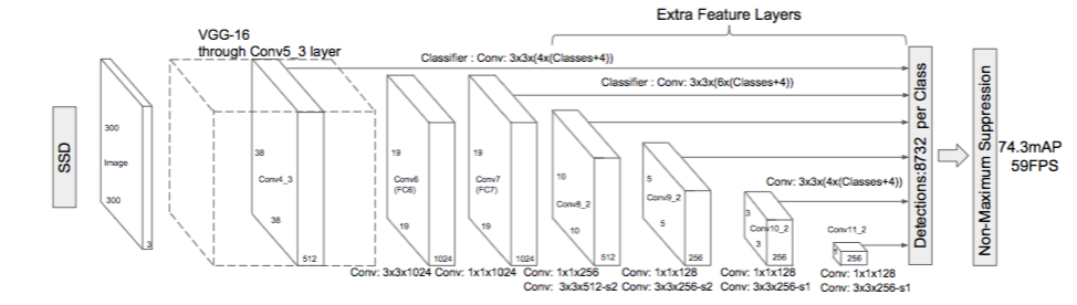
Both YOLO and SSD take a 4D tensor (with batch dimension) during training and a 3D tensor during inference. For the sake of simplicity, I assume that the model takes a tensor of shape (C * H * W) as input. That’s the easy part; almost every computer vision model does that. What about the output?
SSD embraces the idea of multiscale detection; hence, at each of the last layers, it produces a set of predictions. Given an image of input 1 x 300 x 300 x 3, this creates a set of outputs:
Say for example, at Conv4_3, the output is 38×38×4×(c+4).
In terms of number of bounding boxes, there are 38×38×4 = 5776 bounding boxes.
Similarly for other conv layers:
Conv7: 19×19×6 = 2166 boxes (6 boxes for each location)
Conv8_2: 10×10×6 = 600 boxes (6 boxes for each location)
Conv9_2: 5×5×6 = 150 boxes (6 boxes for each location)
Conv10_2: 3×3×4 = 36 boxes (4 boxes for each location)
Conv11_2: 1×1×4 = 4 boxes (4 boxes for each location)
The first version of YOLO doesn’t give a damn about multiscale. The last conv layer produces a fixed set of outputs: there are 7×7 locations at the end with 2 bounding boxes for each location, so YOLO only has 7×7×2 = 98 candidates. This is one reason why early versions of YOLO can be unstable, especially on video streams: it can detect an object well in one frame and fail in the next with almost no difference between the two. The huge number of anchor boxes in SSD contributes a lot to its stability when working with video.
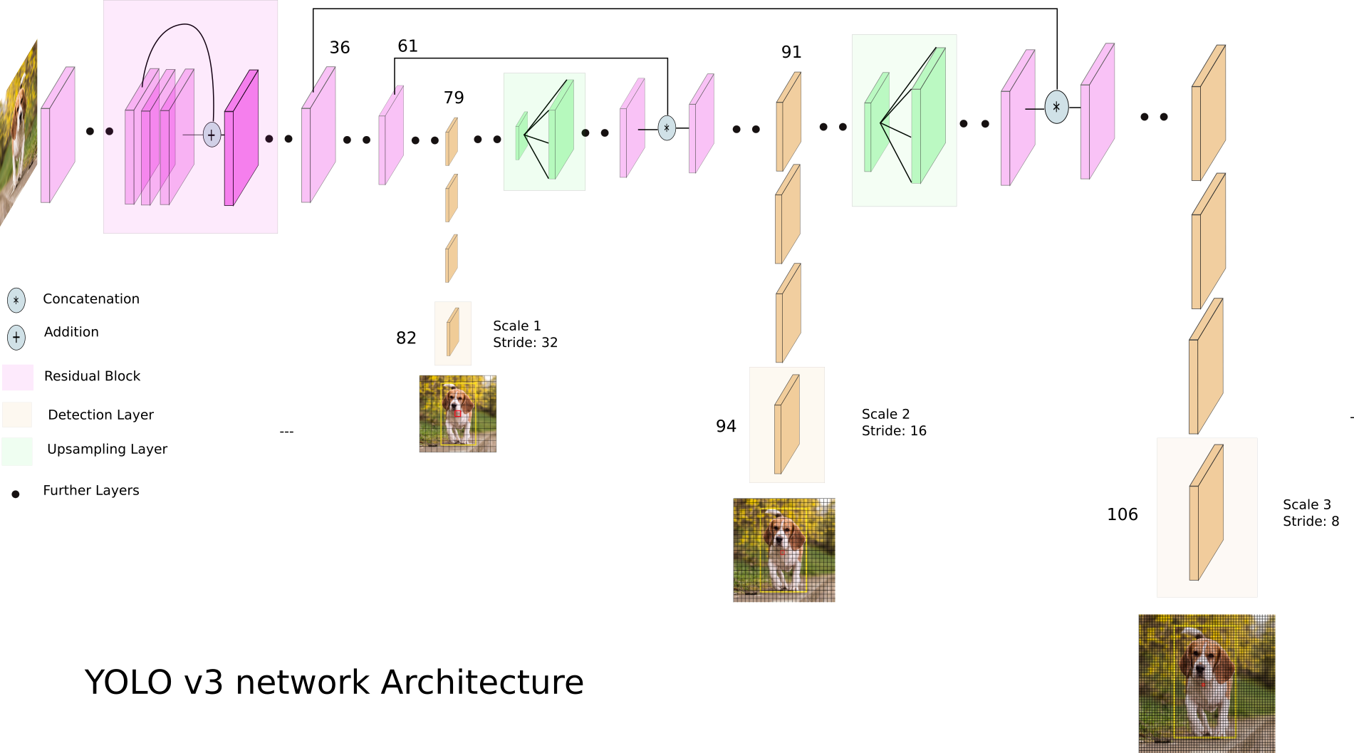
That’s the reason why YOLOv3 implements multiscale detection. With an image of input 1 x 416 x 416 x3,
this creates an output in the form of a list of 3 tensors: [(1 x 13 x 13 x 125), (1 x 26 x 26 x 125), (1 x 52 x 52 x 125)].
Why 125 here?
Suppose for each grid cell we predict 5 bounding boxes, and the dataset has 20 classes. Each bounding box outputs (4 coords + 1 objectness + 20 class scores), so (20 + 5) * 5 = 125.
Another thing is that while SSD considers background as a class, YOLO uses an objectness score, which indicates the probability there is an object in this grid cell (and, depending on the version, that the predicted box overlaps a real object). It’s more intuitive, in my opinion. Treating background as a class can lead to imbalance between this class and the others and this is only partially remedied by hard negative mining. In short, in YOLO it’s 20 + 4 + 1, while in SSD it’s 21 + 4.
Basically speaking, the format of outputs is relatively the same between SSD and YOLO. There are some mismatches in the number of anchor boxes, the exact meaning/parameterization of coordinates, and how objectness is defined. But I believe it’s safe to say the overall structure is similar.
II. Loss function
I believe the second most important factor of a machine learning algorithm is its loss function. While input/output is the core of inference (I think), the loss function is the heart of the training process. In fact, understanding the loss function and how it associates the model output to the label is the only thing I deem important when training a model.
Up until now, you can see that when we compute the forward-pass, we keep mentioning the number of anchor boxes per cell to calculate the total number value each cell must output. However, other than that, we don’t use them at all, we don’t know where they are, their coordinates. So when do we use them?
The answer is: we use them during loss computation and inference. Basically, an object detector doesn’t predict the bounding boxes directly like most people assume; instead it predicts (1) whether an anchor/slot is responsible for an object, and (2) offsets that transform an anchor box into the final bounding box. That’s why we only need the anchor box information when computing loss and during inference. Remember: anchor box + prediction = bounding box.
From the annotation, SSD and YOLO build their ground-truth labels. A label tends to have 5 values: 4 coordinates + class info. They also share the idea of matching anchor boxes to ground-truth boxes. Roughly speaking, the anchor boxes are divided into 2 groups: positive and negative. The positive group includes boxes that have IoU with ground truth bigger than a specified threshold (and vice versa). Each anchor box is typically associated with only one ground-truth box or nothing at all (background). And the model predicts the correction (offsets) of coordinates and the class label for each anchor box. I call it correction because the model doesn’t predict the coordinates directly, but the differences between an anchor box and its corresponding ground-truth box.
Furthermore, as you can see, YOLO and SSD interpret objectness score differently, hence, the loss function will be different too.
To be more specific, here is SSD loss function:
\[L(x, c, l, g) = \frac{1}{N}(L_{conf}(x, c) +\alpha L_{loc}(x, l, g))\]In short, SSD’s loss function is formed by 2 sub-losses: location loss and classification loss. The first one learns the location correction (offset regression), and the second one predicts the class of the box. In the original SSD paper, the location loss is Smooth L1, and the confidence loss is softmax cross-entropy over (N+1) classes (including background).
About YOLO’s loss function:
\[\lambda_{coord}\sum_{i=0}^{S^2} \sum_{j=0}^{B} \mathbb{1}_{ij}^{obj} \left[(x_i - \hat{x}_i)^2 + (y_i - \hat{y}_i)^2\right] + \\ \lambda_{coord}\sum_{i=0}^{S^2} \sum_{j=0}^{B} \mathbb{1}_{ij}^{obj} \left[(\sqrt{w_i} - \sqrt{\hat{w}_i})^2 + (\sqrt{h_i} - \sqrt{\hat{h}_i})^2\right] + \\ \sum_{i=0}^{S^2} \sum_{j=0}^{B} \mathbb{1}_{ij}^{obj} (C_i - \hat{C}_i)^2 + \\ \lambda_{noobj}\sum_{i=0}^{S^2} \sum_{j=0}^{B} \mathbb{1}_{ij}^{noobj} (C_i - \hat{C}_i)^2 + \\ \sum_{i=0}^{S^2} \mathbb{1}_{i}^{obj} \sum_{c \in classes} (p_i(c) - \hat{p}_i(c))^2\]The equation above is the classic YOLOv1 objective. Basically, there are 3 components: location loss, classification loss, and objectness classification. In YOLOv1, the authors used squared error (L2) for all of them (including class probabilities), plus a few coefficients like $\lambda_{coord}$ and $\lambda_{noobj}$ to balance terms.
In later YOLO versions (YOLOv2/v3 and most modern detectors), the practical loss is closer to the following decomposition:
- Box regression: learn offsets (center + size) relative to an anchor (often MSE/SmoothL1, or IoU-based losses in newer versions).
- Objectness: binary classification per anchor (almost always BCE).
- Class prediction: multi-label BCE in YOLOv3 (since it uses independent sigmoid outputs per class).
YOLOv3 loss: what actually happens in code
The confusing part of YOLOv3 is not the final loss formula, but the target assignment / label building (i.e., mapping sparse ground truth boxes into dense feature maps).
At a given detection scale (e.g. 13×13), the model outputs for each grid cell and each anchor:
- 4 numbers for box geometry (encoded as center + width/height)
- 1 objectness score
- $C$ class logits (sigmoid)
During loss computation, YOLOv3 does roughly this (matching the typical PyTorch implementation):
- Assign each ground-truth box to exactly one anchor at exactly one grid cell
- Convert GT box center into grid coordinates.
- Choose the best anchor (highest IoU in width/height space) among the anchors of that scale.
- Mark that (cell, anchor) as responsible for this GT (this is why YOLO targets are very sparse).
- Build masks for positives and negatives
obj_maskis 1 only at responsible (cell, anchor).noobj_maskis 1 everywhere else.- To avoid over-penalizing good predictions, if an anchor has IoU >
ignore_threswith some GT, YOLO setsnoobj_mask = 0there (ignore those negatives).
- Encode the regression targets $(t_x, t_y, t_w, t_h)$
- $t_x, t_y$ are the offsets within the grid cell (fractional part of the GT center in grid coordinates).
- $t_w, t_h$ are log-scale ratios to the anchor size, e.g. \(t_w = \log\left(\frac{w_{gt}}{w_{anchor}}\right),\quad t_h = \log\left(\frac{h_{gt}}{h_{anchor}}\right).\)
- This matches the decoder at inference time: predicted width/height are exponentiated and multiplied by anchor size.
- Compute losses only where they make sense
- Box regression (x/y/w/h) is computed only on positives (
obj_mask). - Objectness is computed on both positives and negatives, but with a much larger weight on negatives in many implementations.
- Classification is computed only on positives.
- Box regression (x/y/w/h) is computed only on positives (
One typical breakdown looks like:
loss_x, loss_y, loss_w, loss_h: MSE on positivesloss_conf: BCE on positives + (scaled) BCE on negativesloss_cls: BCE on positives
This also explains why YOLO can train without explicit hard negative mining like SSD: it relies on (a) sparse positives, (b) an ignore region, and (c) different weights for positive/negative objectness.
As you can see, since the number of anchor boxes in SSD is much larger than in YOLO (especially compared to YOLOv1), the imbalance between positive and negative groups can be more severe in SSD. SSD tackles this with hard negative mining (keep only the hardest negatives up to some ratio like 3:1), while YOLO-style detectors often rely more on loss re-weighting + ignore regions.
III. Conclusion
That’s basically it. In my opinion, these points are the main differences between SSD and YOLO. As it turns out, these two architectures are quite alike. I guess that’s one reason why SSD has remained relatively stable for years, while YOLO progressed massively throughout the years. YOLO is more optimized by design (fewer candidates per scale, the existence of objectness score, etc.) and it’s quite easy for YOLO to adopt SSD’s nice features like multi-scale detection. And eventually, these two original architectures converge into later versions of YOLO.
Furthermore, they also try to leverage other techniques like data augmentation to boost the performance of YOLO.
Other than that, I haven’t seen any improvement of architecture for the last couple of years. Let’s see any progresses to be made in this area in the future. I’ve heard about Nano-Dets and the use of Transformer but it’s for another day.